1 Welcome to R!
R is a computer programming language that is increasingly used for ‘data science’, that is, the manipulation, summarization, and visualization of large datasets. Data comes in many shapes and sizes, however this course is designed to teach you the skills to work with tabular data (rows and columns) such as is often handled in Microsoft Excel.
An example of ‘tabular data’ is shown below. This data concerns different models of car, which we will return to later.
## # A tibble: 6 x 11
##   manufacturer model displ  year   cyl trans      drv     cty   hwy fl    class
##   <chr>        <chr> <dbl> <int> <int> <chr>      <chr> <int> <int> <chr> <chr>
## 1 audi         a4      1.8  1999     4 auto(l5)   f        18    29 p     compact
## 2 audi         a4      1.8  1999     4 manual(m5) f        21    29 p     compact
## 3 audi         a4      2    2008     4 manual(m6) f        20    31 p     compact
## 4 audi         a4      2    2008     4 auto(av)   f        21    30 p     compact
## 5 audi         a4      2.8  1999     6 auto(l5)   f        16    26 p     compact
## 6 audi         a4      2.8  1999     6 manual(m5) f        18    26 p     compact
1.1 A look around RStudio
To get the best out of R, we recommend using the RStudio software which you should now have installed on your computer.
Open RStudio. You will see 3 windows (aka ‘panes’). Each window has a different function.
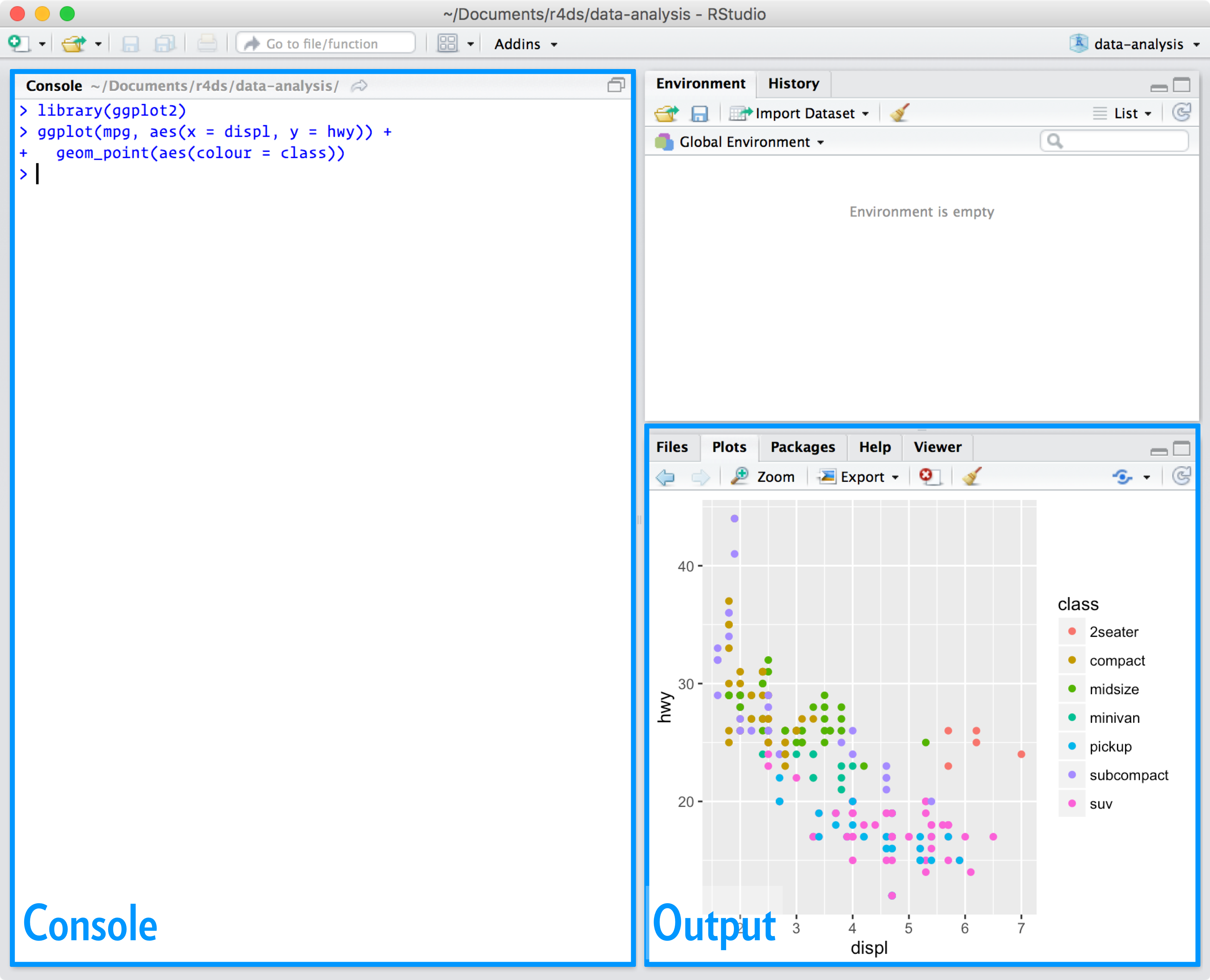
1.2 Console Pane
On the left hand side you have the ‘console’. You can enter commands (code that R can ‘understand’) in this window, and you will get a response to your commands (‘output’) here too. The console is useful for trying out code, but will not save any of your code, so we don’t recommend that you use it exclusively.
1.3 Environment/History Pane
At the top right is the environment pane. Data that you create, or that you import from other places, will be listed here. This data is available for you to access at any time while your RStudio session is open. It is therefore said to be ‘in the working environment.’
The History pane contains a list of commands you have previously entered.
1.4 Plotting Pane
At the bottom right is the plotting (‘Plots’) pane. Here you can immediately see the results of the R code you use to make graphs/charts. There are other tabs here as well which we will introduce later.
1.5 Open a new R script
Because we want to save our code to return to and build on, or use to refresh our memory later, we want to save it in a text file.
I recommend that you create a folder on your Desktop named WEHI_tidyR_course
Go to File > New File > R Script. A new pane will appear at the top left. Save this empty text file as ‘Week_1_tidyverse.R’ within the new Desktop folder.
From now on we will type commands in to the text file, and see the results of our commands either in the console pane, or the plotting pane.
1.7 Executing commands
Executing commands, also called ‘running code’ is the process of submitting a command to your computer, which does some computation and returns an answer. There are a few ways to do this in RStudio. We can:
- select the line(s) of code using the mouse, and then click ‘Run’ at the top right corner of the R text file.
- click anywhere on the line of code and click ’Run
- click anywhere on the line of code and type Cmd + Return (mac), or Ctrl + Return (pc)
We suggest the third option, which is fastest.
When you type in, and then run the commands shown in the grey boxes below, you should see the result in the Console pane at bottom left.
1.8 Simple maths in R
We can use R as a calculator to do simple maths
1 + 100 ## [1] 101More complex calculator functions are ‘built in’ to R, which is the reason it is popular among mathematicians and statisticians.
To use these functions, we first type the function, then enter the number of interest between round brackets.
For example, to take the log or square root of 100:
log(100)## [1] 4.60517sqrt(100)## [1] 10Notice that the ‘square root’ function is abbreviated to ‘sqrt()’. This is to make writing R code faster, however the draw back is that some functions are hard to remember, or to interpret.
1.9 Help!!
To find out more about what a function in R does, add a ‘?’ before the function name, and leave the round brackets empty. Then run the code:
#get help on R functions by using "?"

?sqrt()
You will see the ‘Help’ pane at bottom right springs to life. These help documents give detailed explanations about the function, including how it is used, what input it requires, and, most importantly at the bottom Examples!
You can copy and paste these examples in to your R text file, select and then run them. You should see the output intended by the function authors.
NB don’t worry for now that the sqrt() example is quite complicated. NBB all R ‘functions’ are little programs that were written by other people. There are 1000s of functions available for R, which makes your life simpler because you don’t have to program them all from scratch.
1.10 Variables
A ‘variable’ is a bit of tricky concept, but very important for understanding R. Essentially, a variable is a symbol that we use in place of another value. Usually the other value is a larger/longer form of data. We can tell R to store a lot of data, for example, in a variable named ‘x’.
When we execute the command ‘x’, R returns all of the data that we stored there.
For now however we’ll just use a tiny data set: the number 5. To store some data in a variable, we need to use a special symbol ‘<-’ which in our case tells R to ‘assign the value 5 to the variable x’. This is called the ‘assignment operator’.
Let’s see how this works
# create a variable called 'x', that will contain the number 5.

x <- 5
R won’t return anything in the Console, but note that you now have a new entry in the ‘Environment pane’. The variable name is at the left (‘x’) and the value that is stored in that variable, is displayed on the right (5).
We can now use ‘x’ in place of 5:
x + 20## [1] 25x * 50## [1] 250Can you work out what the * symbol is used for in R?
1.10.1 A note on variables
Variables are sometimes referred to as ‘objects’. In R there are different conventions about how to name variables, but most importantly they:
- cannot begin with a number
- should begin with an alphabetical letter
Variables are also case sensitive:
X## Error in eval(expr, envir, enclos): object 'X' not foundAs we can see, ‘x’ is not the same as ‘X’.
Variables can take any name, but its best to use something that makes sense to you, and will likely make sense to others who may read your code.
R_at_WEHI <- 100For example, this code will work, but is not very intuitive to humans:
log(R_at_WEHI)## [1] 4.60517You may be wondering “why bother with assigning variables, when its less text to type ‘100’?”
This is because we can store huge amounts of data in a single variable. For example, we can store a list of 50 numbers in a variable, and do maths on them all at once.
First we create a list of 50 numbers, using a quick trick ‘1:50’ which means ‘every whole number from 1 to 50’.
Let’s make a variable called ‘long_x’ that stores 1:50.
long_x <- 1:50Now we can multiply every number by 10
long_x * 10## [1] 10 20 30 40 50 60 70 80 90 100 110 120 130 140 150 160 170 180 190 200 210 220 230 240 250 260 270 280 290 300 310 320 330 340
## [35] 350 360 370 380 390 400 410 420 430 440 450 460 470 480 490 500Here we are accessing the power of R, which is designed to do lots of computations based on a single line of code.
1.11 Vectors
In making the long_x variable, we are making a ‘vector’. In this case, it is a sequence of numbers. A technical definition for a vector is ‘a sequence of values of the same data type.’
To better understand this we need to think about ‘types of data’.
The three data types we need to understand for now are:
- numbers (‘numeric’)
- words (‘characters’), and
- TRUE/FALSE (‘logical’)
For example, whole numbers can be added, subtracted and so forth. This ‘numeric’ data type is qualitatively different to a word. Words hold meaning, but can’t be sensibly used in a mathematical equation. TRUE and FALSE have specific, logical meaning for computers. Most of what we do in R is turned into TRUE/FALSE problems which are evaluated ‘under the hood.’
1.11.1 Creating numeric vectors
Above we used a shortcut to create a vector of 50 numbers ( 1:50 ). Ordinarily, we need to enclose values in brackets, separated by commas. The values also need to be ‘concatenated’ using a function called c().
#This new variable will contain a vector of numbers, which in this case is a concatenation of 5, 12 and 22.

numeric_vector <- c(5,12,22)
1.11.2 Character vectors
Character values are written in quotation marks, and character vectors are also constructed using c().
char_vector <- c('dog','cat','pigeon')What happens when you add a character vector to a numeric vector?
numeric_vector + char_vector ## Error in numeric_vector + char_vector: non-numeric argument to binary operatorNothing sensible. R will return an error.
1.11.3 Logical vectors
Finally we can create a vector of logical values. Note that for TRUE and FALSE (always in upper case), quotation marks aren’t used. Here we create a vector of three logical values:
logi_vector <- c(TRUE,TRUE,FALSE)TRUE and FALSE appear in coloured text, indicating that they have a special meaning in the R language.
What happens when we add logical data to numeric data?
numeric_vector + logi_vector## [1] 6 13 22Can you work out how R has calculated this answer?
Essentially, the logical data has been automatically converted to numeric data.
The TRUE values become 1, and FALSE become 0.
Another thing to note is that the values in the vector have been added in their respective orders:
position1: 5 + 1 = 6
position2: 12 + 1 = 13
position3: 22 + 0 = 22
This is called ‘type coercion,’ which we’ll return to later.
1.12 Packages
As mentioned above, many developers have built 1000s of functions and shared them with the R user community to help make everyone’s work easier and more efficient. These functions (short programs) are generally packaged up together in (wait for it) ‘Packages’. For example, the ‘tidyverse’ package is a compilation of many different functions, all of which help with data transformation and visualization. Packages also contain data, which is often included to assist new users with learning the available functions.
To access this wealth of pre-existing functions, we install packages from the Comprehensive R Archive Network (CRAN)
…and if you want the all scripts from The Office (American series) in tabular form, there’s a package for that.
1.12.1 Installing packages
To install a package from CRAN, use the ‘install.packages()’ function:
#install packages using the package names in quotes

install.packages('tidyverse')
This will spit out a lot of text into the console as the package is being installed. Once complete you should have a message
The downloaded binary packages are in... followed by a long directory name.
To access the package functions in our RStudio session, we load the package like so:
#load packages using library(package_name), and drop the quotes

library(tidyverse)
Note that to install a package requires the package name in quotations. Once installed, to load it we drop the quotation marks.
1.13 The pipe %>%
When using functions provided in the tidyverse package, we suggest to write your commands from left to right. This makes reading, and finding bugs in the code, a lot easier. To write code in this way requires a specific symbol, called the pipe which allows the code to be processed in a left-right manner.
The pipe symbol looks like this: %>%
It is a pain to type manually, so we suggest you use a shortcut: CMD + SHIFT + M (mac) or CTRL + SHIFT + M (pc). It takes a little practice, but quickly enables a great increase in your coding speed. The pipe-based method of coding can help new users to become ‘fluent in R’.
Let’s try using the pipe with some data that is packaged up with the tidyverse, called the ‘miles per gallon (mpg)’ data set. This is the data set you saw above, containing information on the mechanical features of different models of car.
First we will assign the currently hidden mpg data set to an explicit variable ‘mpg_df’ in our environment.
mpg_df <- mpgNow we access the contents of mpg_df, and ‘send it into a function’ called head(). The head() function returns the first six rows of a data set (or first six values in a vector) to the console.
#see the first six rows of the mpg data set

#call mpg_df first, then 'send it into' the head function, using the pipe %>%

mpg_df %>% head()
## # A tibble: 6 x 11
## manufacturer model displ year cyl trans drv cty hwy fl class
## <chr> <chr> <dbl> <int> <int> <chr> <chr> <int> <int> <chr> <chr>
## 1 audi a4 1.8 1999 4 auto(l5) f 18 29 p compact
## 2 audi a4 1.8 1999 4 manual(m5) f 21 29 p compact
## 3 audi a4 2 2008 4 manual(m6) f 20 31 p compact
## 4 audi a4 2 2008 4 auto(av) f 21 30 p compact
## 5 audi a4 2.8 1999 6 auto(l5) f 16 26 p compact
## 6 audi a4 2.8 1999 6 manual(m5) f 18 26 p compactNote that unlike the log() and c() functions we used earlier, here the brackets after head() are empty. This still works because the pipe %>% is sending the mpg_df dataset into the head() function.
It has the same outcome as:
head(mpg_df)1.14 Data frames
The final concept we need to understand before starting to make plots in R, are ‘data frames’. The vectors we created above are a simple type of ‘data structure’. Whereas vectors can be thought of as a 1-dimensional data structure (a sequence of values), data frames are a 2D data structure.
Data frames have both rows and columns. Each column is in fact a vector, containing a single type of data. Data frames generally have column names, which we can treat in the same way as a variable.
For example, let’s combine our three vectors into a data frame, using the data_frame() function:
#combine vectors of the same length into a data frame

new_df <- data_frame(numeric_vector, char_vector, logi_vector)new_df## # A tibble: 3 x 3
## numeric_vector char_vector logi_vector
## <dbl> <chr> <lgl>
## 1 5 dog TRUE
## 2 12 cat TRUE
## 3 22 pigeon FALSEImportantly, each column in a data frame must have the same number of values (i.e., the same number of rows).
This will be a familiar data structure for those who use Microsoft Excel, and is very popular in data science.
To make plots in R for this tutorial, we must provide our data in data frame form.
1.6 Comments
When working in R it is very handy to make notes to yourself about what the code is doing. In R, any text that appears after the hash symbol ‘#’ is called a ‘comment.’ R can’t see this text, and won’t try to run it as commands. Comments are useful for reminding your future self what you were aiming to do with a particular line of code, and what was or wasn’t working.
We will use comments extensively in this course.
Try writing your first comment in your R text file (top left panel)