Chapter 25 Now, over to you!
This example has some partial guidelines but ideally you want to attempt this one by yourself and try either a very basic model set up of experiment a bit more using some additional resources that we provided. Let us start together:
#Load language R
library(languageR)
25.1 Data Description
We have some data on realization of the dative as NP or PP in the Switchboard corpus and the Treebank Wall Street Journal collection. Comes with 3263 observations on the 15 variables. We will be replicating the following study:
Bresnan, J., Cueni, A., Nikitina, T. and Baayen, R. H. (2007) Predicting the dative alternation , in Bouma, G. and Kraemer, I. and Zwarts, J. (eds.), Cognitive Foundations of Interpretation, Royal Netherlands Academy of Sciences
#Load the data directly from the package
data(dative)
#If doesnt work, try:
dative<-force(dative)
#Check out the structure and variables that we have in
str(dative)## 'data.frame': 3263 obs. of 15 variables:
## $ Speaker : Factor w/ 424 levels "S0","S1000","S1001",..: NA NA NA NA NA NA NA NA NA NA ...
## $ Modality : Factor w/ 2 levels "spoken","written": 2 2 2 2 2 2 2 2 2 2 ...
## $ Verb : Factor w/ 75 levels "accord","afford",..: 23 29 29 29 42 29 44 12 68 29 ...
## $ SemanticClass : Factor w/ 5 levels "a","c","f","p",..: 5 1 1 1 2 1 5 1 1 1 ...
## $ LengthOfRecipient : int 1 2 1 1 2 2 2 1 1 1 ...
## $ AnimacyOfRec : Factor w/ 2 levels "animate","inanimate": 1 1 1 1 1 1 1 1 1 1 ...
## $ DefinOfRec : Factor w/ 2 levels "definite","indefinite": 1 1 1 1 1 1 1 1 1 1 ...
## $ PronomOfRec : Factor w/ 2 levels "nonpronominal",..: 2 1 1 2 1 1 1 2 2 2 ...
## $ LengthOfTheme : int 14 3 13 5 3 4 4 1 11 2 ...
## $ AnimacyOfTheme : Factor w/ 2 levels "animate","inanimate": 2 2 2 2 2 2 2 2 2 2 ...
## $ DefinOfTheme : Factor w/ 2 levels "definite","indefinite": 2 2 1 2 1 2 2 2 2 2 ...
## $ PronomOfTheme : Factor w/ 2 levels "nonpronominal",..: 1 1 1 1 1 1 1 1 1 1 ...
## $ RealizationOfRecipient: Factor w/ 2 levels "NP","PP": 1 1 1 1 1 1 1 1 1 1 ...
## $ AccessOfRec : Factor w/ 3 levels "accessible","given",..: 2 2 2 2 2 2 2 2 2 2 ...
## $ AccessOfTheme : Factor w/ 3 levels "accessible","given",..: 3 3 3 3 3 3 3 3 1 1 ...Fit the model using a mixture of variables that theoretically are important:
#Fit the model from the paper
dative.glmm <- glmer(RealizationOfRecipient ~
    log(LengthOfRecipient) + log(LengthOfTheme) +
    AnimacyOfRec + AnimacyOfTheme +
    AccessOfRec + AccessOfTheme +
    PronomOfRec + PronomOfTheme +
    DefinOfRec + DefinOfTheme +
    SemanticClass +
    Modality + (1 | Verb), dative,family="binomial", optimizer="nloptwrap",optCtrl=list(maxfun=100000))
## Warning: extra argument(s) 'optCtrl' disregarded## Warning in checkConv(attr(opt, "derivs"), opt$par, ctrl =
## control$checkConv, : Model failed to converge with max|grad| = 0.00405291
## (tol = 0.001, component 1)summary(dative.glmm)## Generalized linear mixed model fit by maximum likelihood (Laplace
## Approximation) [glmerMod]
## Family: binomial ( logit )
## Formula:
## RealizationOfRecipient ~ log(LengthOfRecipient) + log(LengthOfTheme) +
## AnimacyOfRec + AnimacyOfTheme + AccessOfRec + AccessOfTheme +
## PronomOfRec + PronomOfTheme + DefinOfRec + DefinOfTheme +
## SemanticClass + Modality + (1 | Verb)
## Data: dative
##
## AIC BIC logLik deviance df.resid
## 1470.9 1586.6 -716.5 1432.9 3244
##
## Scaled residuals:
## Min 1Q Median 3Q Max
## -7.3502 -0.1899 -0.0689 0.0095 9.6748
##
## Random effects:
## Groups Name Variance Std.Dev.
## Verb (Intercept) 4.693 2.166
## Number of obs: 3263, groups: Verb, 75
##
## Fixed effects:
## Estimate Std. Error z value Pr(>|z|)
## (Intercept) 1.9429 0.6898 2.817 0.004855 **
## log(LengthOfRecipient) 1.2901 0.1562 8.258 < 2e-16 ***
## log(LengthOfTheme) -1.1414 0.1103 -10.346 < 2e-16 ***
## AnimacyOfRecinanimate 2.1918 0.2698 8.124 4.51e-16 ***
## AnimacyOfThemeinanimate -0.8890 0.4969 -1.789 0.073620 .
## AccessOfRecgiven -1.2409 0.2276 -5.453 4.95e-08 ***
## AccessOfRecnew 0.2744 0.2474 1.109 0.267379
## AccessOfThemegiven 1.6303 0.2768 5.890 3.86e-09 ***
## AccessOfThemenew -0.3957 0.1948 -2.031 0.042224 *
## PronomOfRecpronominal -1.5585 0.2495 -6.245 4.23e-10 ***
## PronomOfThemepronominal 2.1458 0.2680 8.006 1.19e-15 ***
## DefinOfRecindefinite 0.7911 0.2089 3.787 0.000153 ***
## DefinOfThemeindefinite -1.0695 0.1990 -5.374 7.69e-08 ***
## SemanticClassc 0.4002 0.3798 1.054 0.292105
## SemanticClassf 0.1344 0.6311 0.213 0.831291
## SemanticClassp -4.0995 1.4748 -2.780 0.005442 **
## SemanticClasst 0.2548 0.2155 1.182 0.237130
## Modalitywritten 0.1318 0.2099 0.628 0.530074
## ---
## Signif. codes: 0 '***' 0.001 '**' 0.01 '*' 0.05 '.' 0.1 ' ' 1##
## Correlation matrix not shown by default, as p = 18 > 12.
## Use print(x, correlation=TRUE) or
## vcov(x) if you need it## convergence code: 0
## Model failed to converge with max|grad| = 0.00405291 (tol = 0.001, component 1)You should get a warning that will tell you that the model has not converged. This is due to optimizer selection. There are variety of those and some can be more complex than others and consequently will require greater availability of computational power. You can read more here. In general, you will note that the estimates will not change as you are changing optimizer but in the ideal scenario you do not want to have any warnings.
Lets now check what our predicted probabilities.
#You can again use the magic of plot_model
plot_model(dative.glmm, type='eff')
## $LengthOfRecipient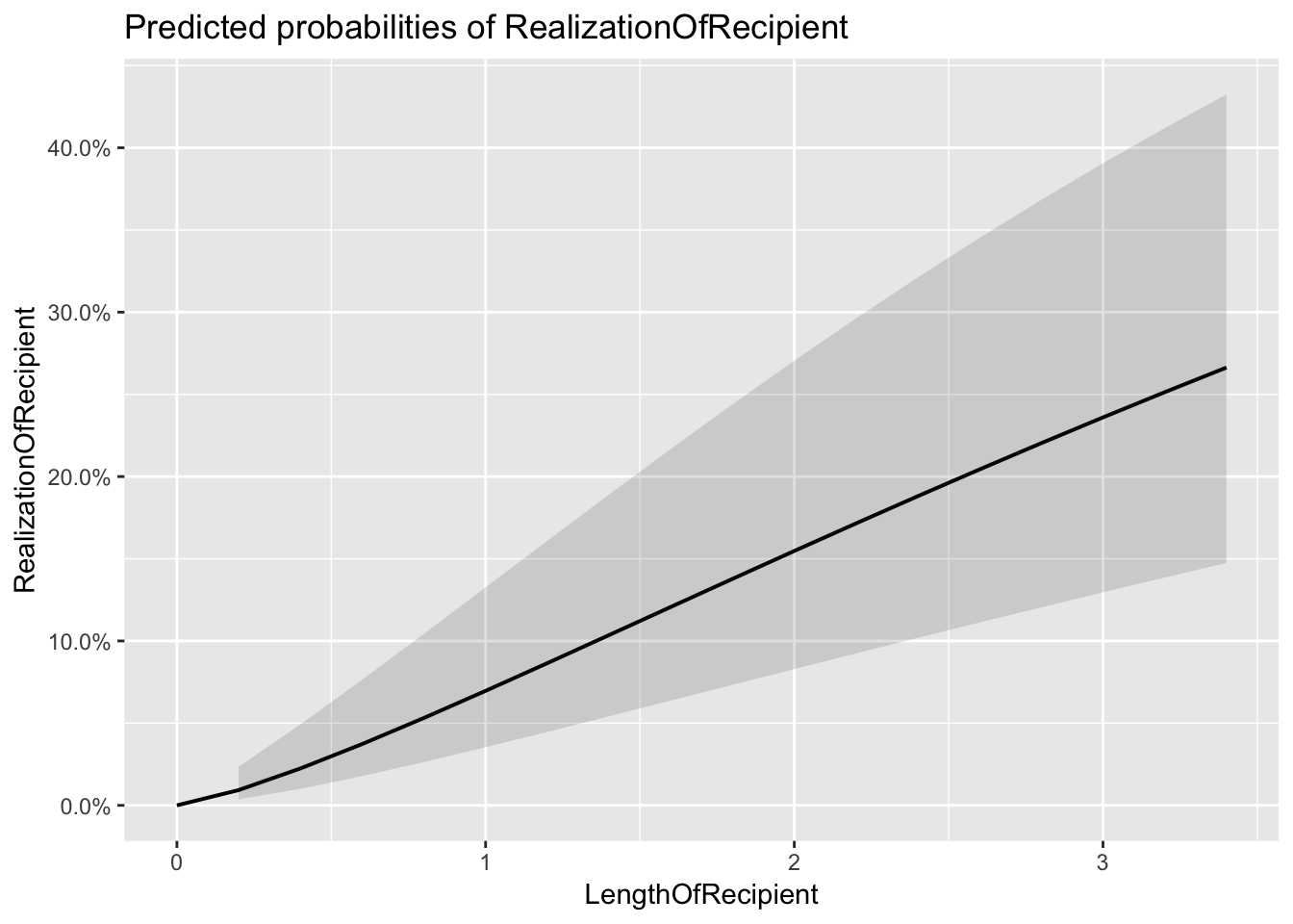
##
## $LengthOfTheme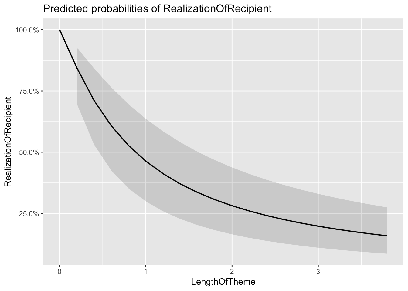
##
## $AnimacyOfRec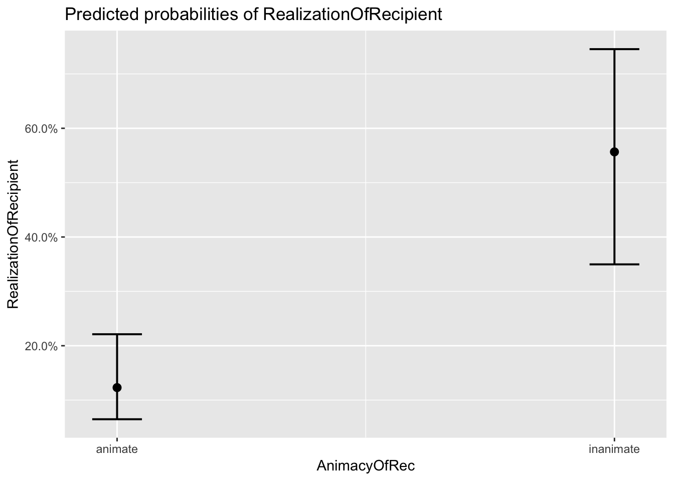
##
## $AnimacyOfTheme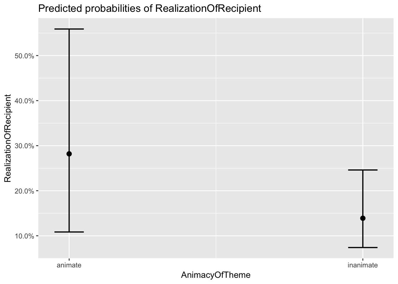
##
## $AccessOfRec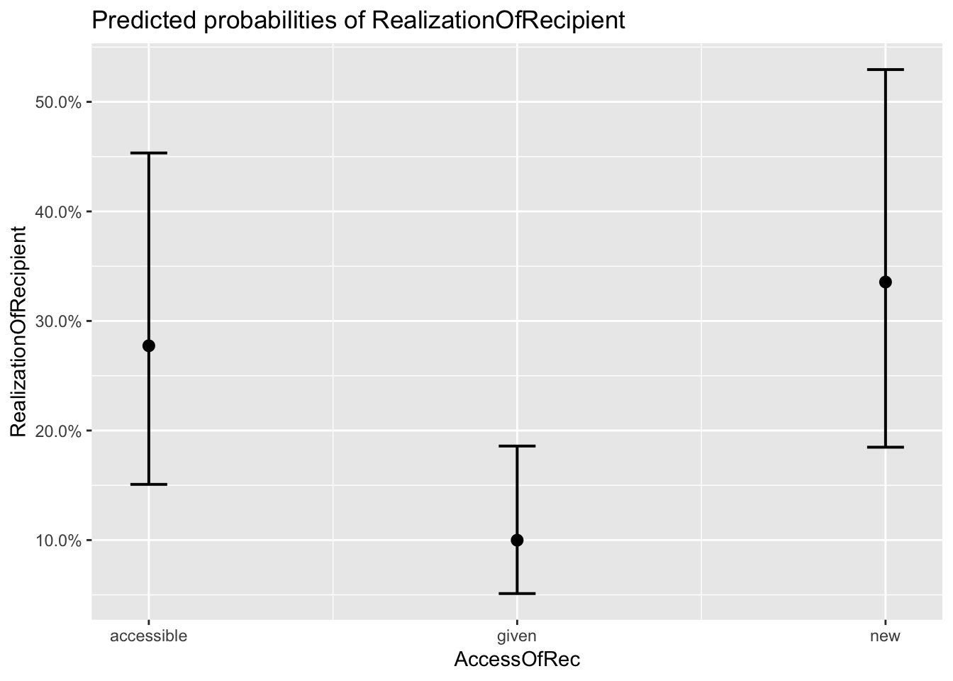
##
## $AccessOfTheme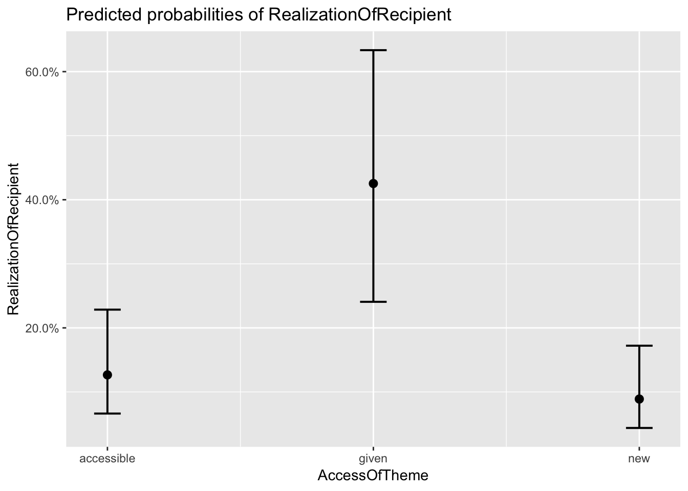
##
## $PronomOfRec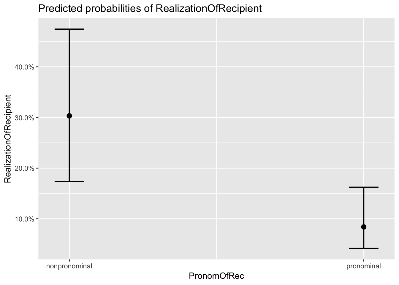
##
## $PronomOfTheme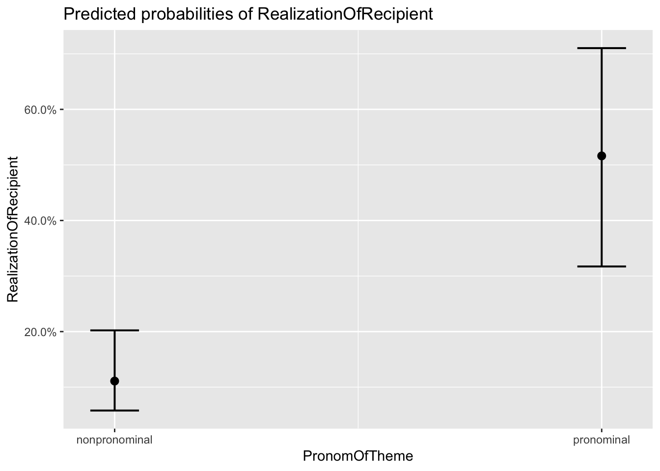
##
## $DefinOfRec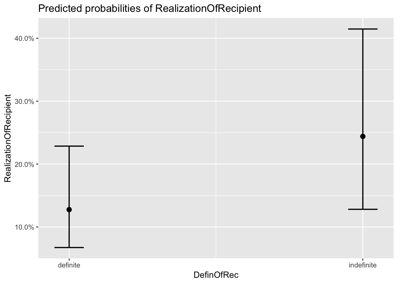
##
## $DefinOfTheme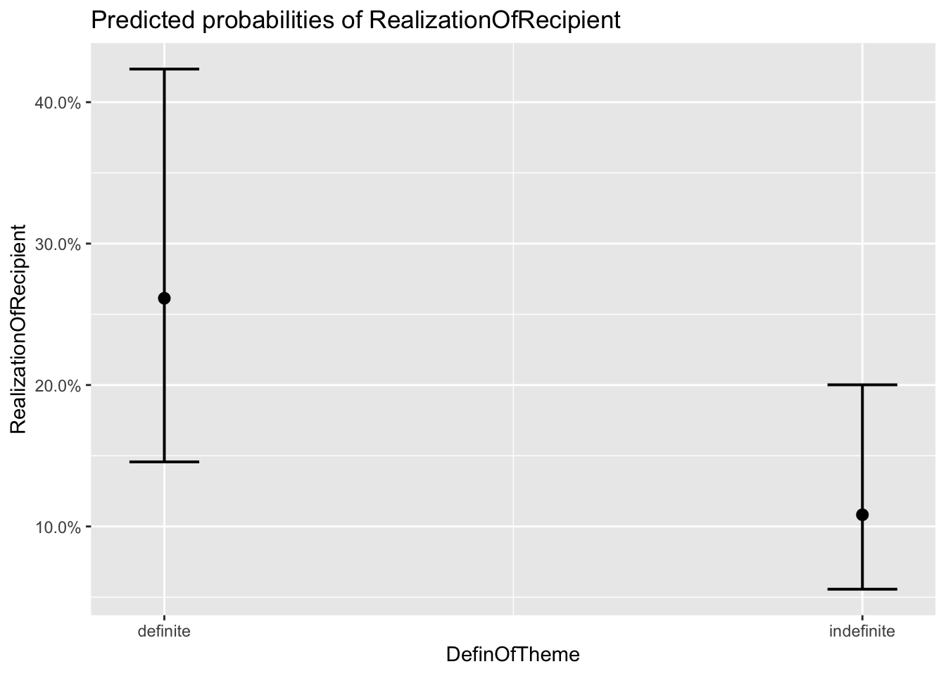
##
## $SemanticClass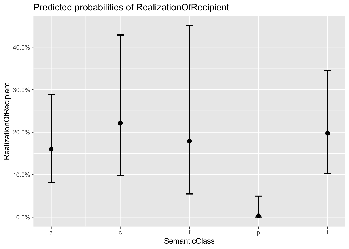
##
## $Modality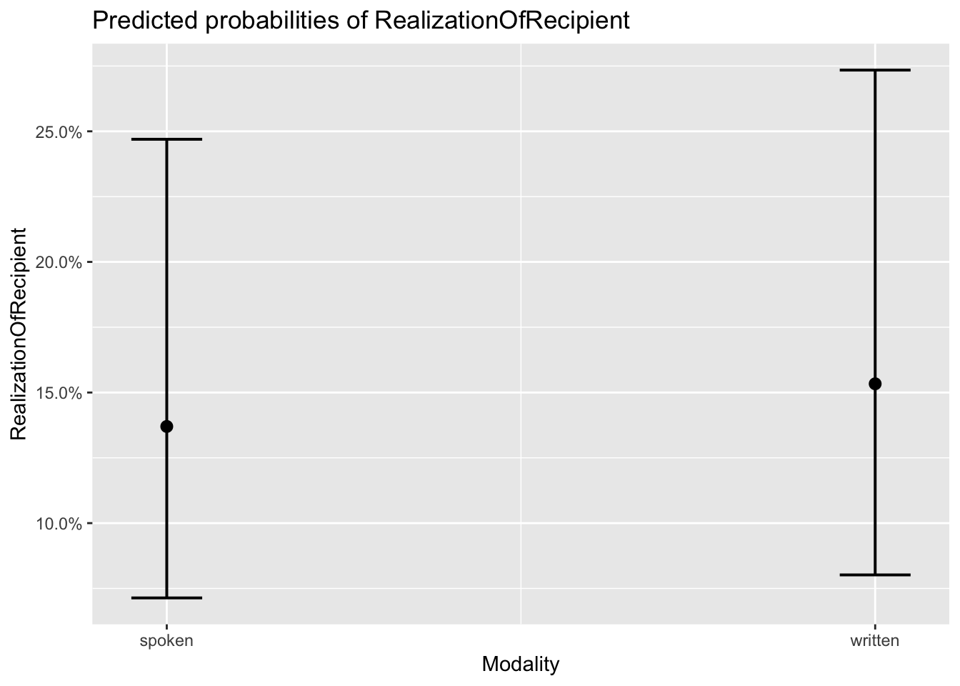
Now by yourself you can work through two examples (one for lmer() and one for glmer())
#Present and investigate the results
#Design a null model to perform a model selection - you can experiment here with other variables or model types
#Produce final results for nice table in texreg
#Transform coefficients and compare the odds (final model)
#Provide a confusion matrix and calculate the ratio of correctly predicted cases
#Provide some nice plots to accompany your results
#Save the script-save the plots
Check out these further resources to see even more examples of application and various outputs you can get to in glmer(). The list is in fact growing and will continue to grow making it easier and easier to fit these great models :)
Among many, we recommend:
Linear Mixed Effects
- Bodo Winter: A Very Basic Tutorail For Performing Linear Mixed Effect Analyses
- John Fox: Linear Mixed Models
- Bates et al (2015): Fitting Linear Mixed-Effects Models Using lme4
- Belenky et al (2003): Patterns of performance degradation and restoration during sleep restriction and subsequent recovery: a sleep dose‐response study.
GLMER