3 Open research approach
Our lab is committed to transparent and reproducible research. This page describes our default process for conducting and reporting quantitative research. All lab members are invited to improve the documentation for our current process and suggest ways to improve our process.
3.1 Overview
Each project is maintained in a self-contained directory (folder) using a standard template for organization. This contains folders for data, code scripts, output, and the manuscript. We use Github for version control and collaboration. We write manuscripts using R-markdown, typically knitting to Microsoft Word to enable sharing and revisions with non-programmer colleagues. R-markdown documents can include code chunks in R and in Python. Upon publication, we create a DOI-indexed copy of our Github repository, which includes all analytic code and data except for sensitive data that must be kept confidential.
3.2 R and Rstudio
R is a free, open-source programming language commonly used in statistics, data science, and quantitative research. R studio is the most popular integrated development environment (IDE) for use with R. We use R and Rstudio for much of our work: to analyze data, program models, and write reproducible manuscripts. Our lab website and lab manual were both created in Rstudio as well. RStudio can also be used for Python, if you install Python and point RStudio to it.
3.3 Rstudio project & folder organization
Rstudio projects are the recommended method for keeping all data, scripts, and output for a project in a single place. An Rstudio project is linked to a specific working directory. In our lab, we have a template we use for each project, with a set file structure. Typically, one project = one academic paper (that way, when we go to publish, we can easily publish the accompanying project directory). The generic project directory template is not on Github because if we added it, the .gitignore file and the ignored folders/files would not show up. Ask Alton to share our generic project directory with you.
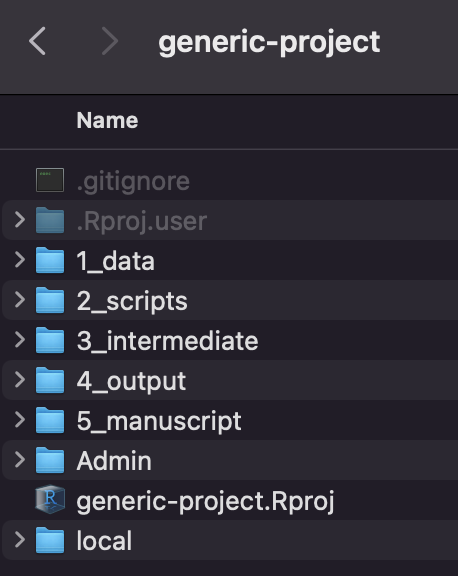
The directories in our generic project are:
1_data folder containing all raw data, before any code has been applied, as well as tables of model parameters that are estimated from the literature or other sources. Often, we will include sub-directories within data with information on the data sets (e.g., data dictionaries or keys).
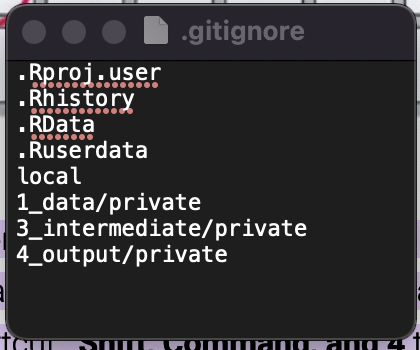
Note: We generally do not upload private line-level data on individual patients into GitHub or publish these data. If you are using an encrypted laptop or a MCHI desktop computer, you can, in most cases, keep line-level data in a sub-directory on your computer (encrypted laptop or MCHI desktop) named “private”. The .gitignore file dictates that the private directory will not be version controlled using Git nor uploaded to Github. This is to comply with data use agreements and avoid improper disclosure of private data. If another team member who has permission wants to work on the project on their own computer, they can first clone the project from Github, but this will not include the ‘private’ directory. They will then need to transfer the data via an approved secure method and create the private directory on their own machine before the data will load.
2_scripts folder for storing all scripts. The preferred naming convention for your scripts is to start with a 2-digit number and underscore, followed by a brief description of what the script does. Often, we have an additional script that contains helper functions which may be shared across scripts. For example, the files in your scripts folder may look like:
- 00_helper-functions.R
- 01_data-cleaning.R
- 02_prediction-model-dev.R
- 03_prediction-model-calibration.R
- 04_results-analysis.R
Every script should be written such that it can run successfully in a new R session with no variables in the environment. At the beginning of the script, any necessary packages should be loaded, any necessary data should be read in from file (e.g., from the 1_data or 3_intermediate folders), and if any scripts containing helper functions should be run (e.g., using
source(./2_scripts/00_helper-functions.R)).3_intermediate this folder can be used if you have intermediate output that is primarily meant as an input to another script or function, rather than to be analyzed or graphed. For example, you could store an .RDS file of a model or data structure that is generated in one script and then analyzed in another.
Note there is also a private sub-directory in the intermediate folder. This is for any datatable or object that contains line-level data that cannot be shared publicly. For example, you may process the raw data in the 1_data/private folder and then put a clean version in the 3_intermediate/private folder. Note that some RObjects you wouldn’t necessarily expect actually contain line-level data (for example, a nested cross validation object or machine learning model, depending on how they are generated, could have line-leve data embedded in them).
4_output this folder will contain the output from your scripts, such csv files containing a table of simulation model output or figures. Again, any output with line-level data should be saved in the 4_output/private.
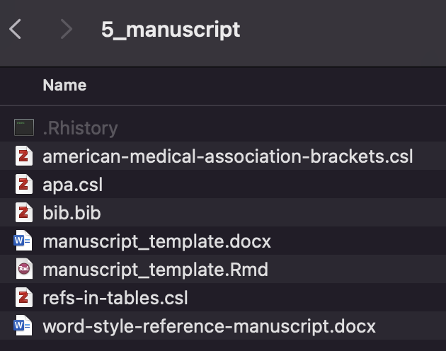
5_manuscript this folder contains the Rmarkdown file in which you write the manuscript, a .bib file containing the references, a Word reference file, and it will contain the most current Word document of the paper at any given time.
In addition, the generic project has a .gitignore file, which specifies which directories should not be tracked via Git (and therefore will not be uploaded onto Github). If you add a subdirectory you want to keep outside of Github, you can add it to this file as a new line.
3.3.1 Relative referencing
When reading or writing files, many new programmers are tempted to either (A) write the full path to the file every time, or (B) use the set working directory command at the start of their script, like this:
fread(\"C:\Users\alton\OneDrive - McGill University\Projects\generic-project\1_data\data.csv")
or
setwd(\"C:\Users\alton\OneDrive - McGill University\Projects\generic-project\1_data\")
fread("data.csv")
The problem with these approaches is that your code isn’t transportable; if you move the project directory anywhere else, or if someone else tries to run it on their computer, the links will break. Instead, all paths should be defined relative to the project’s root directory (the directory where your .rproj file is). Like this:
Create an Rstudio project
fread(1_data\data.csv)
3.4 Project management with Rstudio and Github
While it takes a little effort to set up, Git, Github, and RStudio all play well together. To get started, install git (and R + RStudio if you haven’t), and create a free Github account. The guides below should help you get set up. Once you have a project playing nicely with Github, you’ll want to get in the habbit of commiting and pushing changes every time you work on the project with a meaningful commit message. If it’s a collaborative project, you also want to make sure and pull changes everytime you start working to make sure you have the most recent updates.
On your encrypted laptop or MCHI desktop, you can cache a Github personal access token to avoid having to enter your credentials everytime you interact with Github. Use the resources below and/or search the web to figure out how.
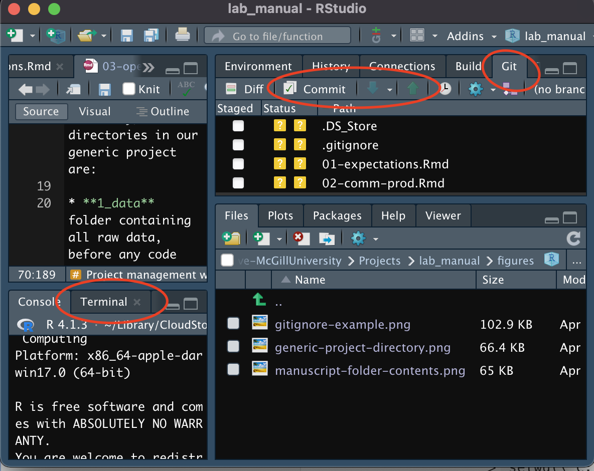
The easiest way to interact with Github on an Rstudio project is using the Git panel to pull the latest version from Github to your computer, then commit and push any changes you make back onto Github. Sometimes, if you run into challenges or make lots of changes at once, the Git panel can be buggy in those cases you’ll need to use the terminal (or, you could install Github Desktop and try using that).
Resources:
- Using Git within RStudio page on a course website by Benjamin Soltoff is the guide I used to get set up.
- Happy Git and Github for the useR is a fairly comprehensive e-book
- Using personal access tokens with Git and Github by Ed Goad seems to cover the basics for caching your Github credentials.
3.5 Writing manuscripts in Rmarkdown
RMarkdown is a great tool for generating analytic reports. RMarkdown can generate documents programmatically, in a way that plays nicely with Git for version control, and with all of the tables, figures, and numbers generated based on your code. Writing in RMarkdown is slower than writing in a word processor, especially at first. However, if you end up changing one input to your model that impacts all of your results, you can quickly re-run your code and regenerate your document using RMarkdown. If writing in Word, you would need to manually replace every figure, table, and reported quantity that was impacted.
A typical RMarkdown document contains code chunks in which you write R code (or python if configured). They look like this:
```{r setup, include=FALSE}
library(ggplot2)
fread(“1_data/data.csv”)
```
Typically, you’ll have a chunk like this named ‘setup’ at the top of the document where you load packages and apply global settings. Then, you can add code chunks throughout the document to read in and format data, generate figures and tables, and perform calculations. It is possible to conduct the entire analysis and knit the paper from .Rmd file, but this is only recommended for very simple/small analyses. If you find yourself with hundreds of lines of code in the code chunks of your .Rmd file, you may wish to instead move that code into an analysis or helper function script (.R file) that is kept in the \2_scripts directory, instead of in the .Rmd file itself.
You can also include in-line R code to programaticaly generate numbers that show up mid-sentence in your report. For example, this code:

Can creates something like this when the document is knitted:
The mean cost per person was $1,212.
RMarkdown can create HTML, PDF, and Microsoft Word documents. We generally use RMarkdown to generate Word documents, because they are the easiest to revise with collaborators. Our generic project folder contains a starter manuscript, which you can revise to develop your project.
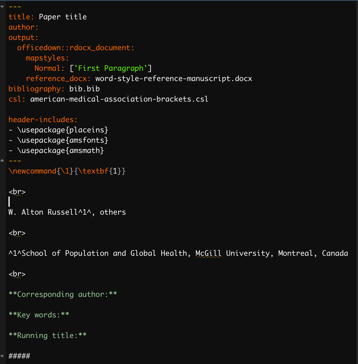
The default template is set to be ‘knit’ into a Microsoft word document, using the citation stype ‘american-medical-association-brackets.csl’ and the bibliography file ‘bib.bib’. Note that you will likely add a different .bib file, generated from Zotero, with a different name. In that case, (1) add your .bib file to the manuscript directory, then (2) change the line bibliography: bib.bib in the .Rmd header to point to your .bib file. If your manuscript involves mathematical equations, you can use Latex and add latex packages to the header under header-includes.

Resources:
- R Markdown Cookbook (2022) by Yihui Xie, Christophe Dervieux, and Emily Riederer is a go-to resource
- RMarkdown for writing reproducible scientific papers (2017) is a helpful blog post by Mike Frank and Chris Hartgerink
- Markdown Cheatsheet by adam-p on github
3.6 Citation management
A good citation management program is essential. Up until now, Alton has used Mendeley, which is a great tool. However, Mendeley is now owned by Elsevier, a large academic publisher with some business practices Alton disagrees with. As such, he is transitioning to Zotero, a free and open source reference manager. Unless you already have a favorite system, we recommend Zotero. A pro-tip: Alton recommends adding the PDF of manuscripts to Zenodo and reading them within Zotero’s PDF reader, which lets you highlight and annotate your files.
To use Zotero for a RMarkdown-based manuscript:
Create a Zotero collection where you add relevant references
You can share this collection with collaborators who use Zotero
You can add the PDFs and highlight/annotate them
For all papers you plan to cite assign a unique citation key
[First authors’ last name] [Publication date] (e.g., Russell2022) is a common structure
Add the text
Citation Key: [your citation key]anywhere in the extra field of the item in Zotero
In Rstudio, use
@and the citation key in brackets wherever you wish to cite a paper.Example for one paper:
[@Russell2021]Example for multiple papers
[@Russell2021; @Russell2021b; @Buckeridge2017]
Place a bibtex (.bib) file for the collection in the
5_manuscriptfile of your project- In Zenodo, right-click a collection and click
Export collection
- In Zenodo, right-click a collection and click
In the YAML header of your .Rmd file, set the bibliography name to the proper filename
- Example:
bibliography: pathogen_inactivation.bib
- Example:
Knit your Rmarkdown document and check that the references generated properly
Replace your .bib file via this process anytime you’ve added or modified references in Zotero.
3.7 Code style and documentation
Most of us are not trained software engineers, but we still aim to create readable code. Collaborators, our future selves, and people trying to build on our work in the future will thank us. Header comments at the top of each script (or code chunk in an RMarkdown file, if it isn’t self-evident from the chunk name) can let readers quickly know the main purpose and output of a script. Function comments at the start of a function should describe the purpose, inputs, and outputs. Section headers and In-line comments can help organize the document and help users understand exactly what does what. Note that while comments are a useful tool, they are no substitute for descriptive variable names and legible code.
Resources:
- The tidyverse style guide by Hadley Wickham
3.8 Publication of data and code
We always publish our full analytic code and any data that we are allowed to make public. Typically we do this by publishing out Github repository to Zenodo (https://zenodo.org/), which creates a DOI (digital object identifier). We then cite this in our publications.
3.9 More resources
- “Putting the R into Reproducible Research” Dr Anna Krystalli, 2019.
- “Project-oriented workflow” Jenny Bryan, 2017.