2 Deep Dive into Linear Algebra

2.1 Definition of Vector Space

Definition: A vector space consists of a set V along with 2 operations “+” (addition) and “*” (scalar multiplication) subject to 10 properties

Example: $L = $ Show L forms a vector under the operations vector addition and vector scalar multiplication.

(i) let $\vec{a}, \vec{b} \epsilon L$

$$\therefore \vec{a} = \begin{bmatrix} x_{1} \\ y_{1} \end{bmatrix} = \begin{bmatrix} x_{1} \\ 5y_{1} \end{bmatrix} = \begin{bmatrix} 1 \\ 5 \end{bmatrix}x_{1}$$

$$\vec{b} = \begin{bmatrix} x_{2} \\ y_{2} \end{bmatrix} = \begin{bmatrix} x_{2} \\ 5y_{2} \end{bmatrix} = \begin{bmatrix} 1 \\ 5 \end{bmatrix}x_{2}$$

$$\Rightarrow \vec{a} + \vec{b} = \begin{bmatrix} 1 \\ 5 \end{bmatrix}x_{1} + \begin{bmatrix} 1 \\ 5 \end{bmatrix}x_{2} = \begin{bmatrix} 1 \\ 5 \end{bmatrix}(x_{1}+x_{2}) \epsilon L$$

(ii) commutative: $$\vec{a}+\vec{b} = \vec{b}+\vec{a}$$

(iii) let $\vec{c} \epsilon L$ $$\therefore(\vec{a} + \vec{b}) + \vec{c} = \vec{a} + (\vec{b} + \vec{c})$$ by associativity of vector (+)

(iv) zero vector: let $x=y=0$ $$\therefore \begin{bmatrix} 0 \\ 0 \end{bmatrix} = \begin{bmatrix} 0 \\ 5 * 0 \end{bmatrix}$$

(v) additive inverse: let $$\vec{d} = \begin{bmatrix} -x_{1} \\ -5x_{1} \end{bmatrix} \epsilon L$$

$$\therefore \vec{a} + \vec{d} = \begin{bmatrix} x_{1} \\ 5x_{1} \end{bmatrix} + \begin{bmatrix} -x_{1} \\ -5x_{1} \end{bmatrix} = \begin{bmatrix} 0 \\ 0 \end{bmatrix}$$

$$\therefore$$ the additive inverse of $$\vec{a}$$ is in L

(vi) let $c \epsilon \mathbb{R}$; $$c \vec{a} = c\begin{bmatrix} x_{1} \\ 5x_{1} \end{bmatrix} = cx_{1}\begin{bmatrix} 1 \\ 5 \end{bmatrix} \epsilon L$$

$$\therefore$$ closed under scalar multiplication

(vii) $$(c_{1}+c_{2})\vec{a} = c_{1}\vec{a} + c_{2}\vec{a}$$ by distributive property of scalar multiplication

(viii) $$c_{1}(\vec{a}+\vec{b}) = c_{1}\vec{a} + c_{1}\vec{b}$$ by distributive property of vector (+)

(ix) $$(c_{1}c_{2})\vec{a} = c_{1}(c_{2}\vec{a})$$ by associativity of scalar multiplication

(x) $$1\vec{a} = \vec{a}$$

Extend to $\mathbb{R^{n}}$

I. $\mathbb{R^{2}}$ (entire space)

II. Any line through origin

III. $\vec{0}$ (trivial space)

Other kinds of vector spaces:

Example: let $P_{2} = \begin{Bmatrix}a_{0}+a_{1}x+a_{2}x^{2} | a_{0},a_{1},a_{2} \epsilon \mathbb{R^{2}}\end{Bmatrix}$ Show $P_{2}$ is a vector space under the operations for addition and multiplication by a constant.

All axioms are easy to check. I’ll show a few.

Closure under addition:

let $f(x), g(x) \epsilon P_{2} \therefore$ $$f = a_{0}+a_{1}x+a_{2}x^{2}$$

$$g = b_{0}+b_{1}x+b_{2}x^{2}$$

$$\Rightarrow f+g= (a_{0}+b_{0})+(a_{1}+b_{1})x+ (a_{2}+b_{2})x^{2} \epsilon P_{2}$$

therefore closed under addition

Closure under scalar multiplication:

let $c \epsilon \mathbb{R}$ $$\Rightarrow cf = c(a_{0}+a_{1}x+a_{2}x^{2})$$

$$= ca_{0}+ca_{1}x+ca_{2}x^{2} \epsilon P_{2}$$ therefore closed under scalar multiplication

Zero element:

let $a_{0}=a_{1}=a_{2}=0 \therefore h(x)=0 \epsilon P_{2}$ and $0 + f(x) = f(x)$

Subspaces

General polynomial space $$P_{n}=\begin{Bmatrix}a_{0}+a_{1}x+a_{n}x^{n} | n \epsilon \mathbb{N}, a \epsilon \mathbb{R^{2}}\end{Bmatrix}$$

$P_{k}$ is a subspace of $P_{n}$ for $0 \leq k \leq n$

Example: let $f(x) = 3x^{2}+2x+1$

$f(x) \epsilon P_{n}$ for $n \geq 2$, $f(x)$ does not span $P_{1}$

 

Calculus Operations:

Example: $V=\begin{Bmatrix}y^{'} + y | y^{'} + y = 0\end{Bmatrix}$ homogeneous ODE

Closure under addition: let $f,g \epsilon V$

$$\therefore f^{'}+f=0, g^{'}+g=0$$ by definition

$$\frac{d}{dx}[f+g]+f+g$$

$$=\frac{df}{dx} + \frac{dg}{dx} + f + g$$

$$=(\frac{df}{dx} + f) + (\frac{dg}{dx} + g)$$

$$= 0 + 0$$

$$= 0 \therefore f+g \epsilon V$$

Closure under scalar multiplication: let $c \epsilon \mathbb{R}$

$$\frac{d}{dx}[cf] + cf$$

$$=c\frac{df}{dx} + cf$$

$$=c(\frac{df}{dx} + f)$$

$$=c * 0$$

$$=0 \therefore cf \epsilon V$$

Zero element: let $h=0$

$$\therefore \frac{dh}{dx} + h = 0+0=0 \therefore \vec{0} \epsilon V$$

Yes, this forms a vector space

Examples of Vector Space Rules:

Closure under Addition:

$$let\ A, B \in V \therefore A= \left[ \begin{array}{cc} a_1 & 0 \\ 0 & a_2 \end{array} \right], \ \ B= \left[ \begin{array}{cc} b_1 & 0 \\ 0 & b_2 \end{array} \right]$$

$$\Rightarrow A + B = \left[ \begin{array}{cc} a_1+b_1 & 0+0 \\ 0+0 & a_2+b_2 \end{array} \right] = \left[ \begin{array}{cc} a_1+b_1 & 0 \\ 0 & a_2+b_2 \end{array} \right] \in V$$

Closure under Scalar Multiplication:

$$let\ c \in \mathbb{R} \therefore cA= c\left[ \begin{array}{cc} a_1 & 0 \\ 0 & a_2 \end{array} \right] = \left[ \begin{array}{cc} ca_1 & c\times0 \\ c\times0 & ca_2 \end{array} \right] = \left[ \begin{array}{cc} ca_1 & 0 \\ 0 & ca_2 \end{array} \right] \in V$$

Zero Element:

$$let\ A=B=0\therefore \left[ \begin{array}{cc} 0 & 0 \\ 0 & 0 \end{array} \right] \in V$$

Example: V=set of singular matrices. Is it a vector space? NO

$$let\ A= \left[ \begin{array}{cc} 1 & 0 \\ 0 & 0 \end{array} \right],\ B= \left[ \begin{array}{cc} 0 & 0 \\ 0 & 1 \end{array} \right]$$

$$A,B\in V\ by\ def^{(n)};\ but, A+B=\left[\begin{array}{cc}1 & 0 \\0 & 1\end{array}\right] \notin V$$

therefore not closed, therefore not a vector space

Complex Numbers

Example: $V=\Bigg\{\left[\begin{array}{cc}1 & 0 \\0 & 1\end{array}\right]\Bigg|\ a,b\in \mathbb{C},\ a+b=0\Bigg\}$

Is this a Vector Space? YES

Closure under Addition:

$$let\ A, B \in V \therefore A= \left[\begin{array}{cc}0 & a_1 \\a_2 & 0\end{array}\right], \ \ B= \left[\begin{array}{cc}0 & b_1 \\b_2 & 0\end{array}\right]$$

$$a_1 + a_2=0,\ \ b_1 + b_2=0,\ \ \therefore \ a_1 + a_2 + b_1 + b_2=0$$

$$\Rightarrow A + B = \left[\begin{array}{cc}0+0 & a_1+b_1 \\a_2+b_2 & 0+0\end{array}\right] = \left[\begin{array}{cc}0 & a_1+b_1 \\a_2+b_2 & 0\end{array}\right]\in V$$

Closure under Scalar Multiplication:

$$let\ c \in \mathbb{C} \therefore c=c_1 + c_2i\ where\ i=\sqrt{-1}$$

$$\therefore cA= (c_1+c_2i)\left[\begin{array}{cc}a_1 & 0 \\0 & a_2\end{array}\right]$$

$$=c_1\left[\begin{array}{cc}0 & a_1 \\a_2 & 0\end{array}\right] +c_2i\left[\begin{array}{cc}0 & a_1 \\a_2 & 0\end{array}\right]$$

$$=\left[\begin{array}{cc}0 & c_1a_1 \\c_1a_2 & 0\end{array}\right] +\left[\begin{array}{cc}0 & c_2ia_1 \\c_2ia_2 & 0\end{array}\right]$$

$$=\left[\begin{array}{cc}0 & ca_1 \\ca_2 & 0\end{array}\right]\in V$$

Zero Element: $$let\ A=B=0\therefore \left[ \begin{array}{cc} 0 & 0 \\ 0 & 0 \end{array} \right] \in V$$

Subspaces & Spanning Sets

Subspaces of $\mathbb{R}^{3}$:

• point($\overrightarrow{0}$)
• line through origin
• plane through origin
• $\mathbb{R}^{3}$

Subspace:

A subspace W of a vector space V is another vector space contained within V; W must be closed under linear combinations

Span:

Let S = $\{\overrightarrow{s_1},\overrightarrow{s_2},...,\overrightarrow{s_n}\}$; the span of S, denoted span$\{$S$\}$ is the set of all linear combinations.

$\therefore$ span$\{$S$\}$ = $\{c_1\overrightarrow{s_1}+...+c_n\overrightarrow{s_n}|c_i\in \mathbb{R},\overrightarrow{s_i}\in S\}$

Example: $let\ \hat{i}=\left[\begin{array}{c}1 \\0 \\0\end{array}\right],\ \hat{j}=\left[\begin{array}{c}0 \\1 \\0\end{array}\right],S=\{\hat{i},\hat{j}\}$

$\therefore span(S)=\{c_1\hat{i}+c_2\hat{j}|c_i,c_2\in \mathbb{R}\}$

$\Rightarrow xy-plane, z=0$

Example: span$\Bigg\{\left[\begin{array}{c}1 \\0 \\0\end{array}\right],\left[\begin{array}{c}0 \\1 \\0\end{array}\right],\left[\begin{array}{c}0 \\0 \\1\end{array}\right]\Bigg\}$=$\mathbb{R}^{3}$

 

 

Example: span$\Bigg\{\left[\begin{array}{c}1 \\0 \\0\end{array}\right],\left[\begin{array}{c}2 \\0 \\0\end{array}\right],\left[\begin{array}{c}3 \\0 \\0\end{array}\right],\left[\begin{array}{c}4 \\0 \\0\end{array}\right]\Bigg\}$=$\Bigg\{\left[\begin{array}{c}1 \\0 \\0\end{array}\right]c\ \Bigg|\ c\in \mathbb{R}\Bigg\}$ = x-axis (line)

 

 

Example: span$\Bigg\{\left[\begin{array}{c}1 \\0 \\0\end{array}\right],\left[\begin{array}{c}0 \\0 \\1\end{array}\right],\left[\begin{array}{c}5 \\0 \\5\end{array}\right]\Bigg\}$=$\Bigg\{\left[\begin{array}{c}1 \\0 \\0\end{array}\right]c_1+\left[\begin{array}{c}0 \\0 \\1\end{array}\right]c_2+\left[\begin{array}{c}5 \\0 \\5\end{array}\right]c_3\ \Bigg|\ c_1, c_2, c_3\in \mathbb{R}\Bigg\}$

$5\left[\begin{array}{c}1 \\0 \\0\end{array}\right]+5\left[\begin{array}{c}0 \\0 \\1\end{array}\right]=\left[\begin{array}{c}5 \\0 \\5\end{array}\right]$, $\therefore \Bigg\{\left[\begin{array}{c}1 \\0 \\0\end{array}\right]c_1+\left[\begin{array}{c}0 \\0 \\1\end{array}\right]c_2\ \Bigg|\ c_1, c_2\in \mathbb{R}\Bigg\}$ = xz-plane

 

 

Solutions to Assorted Problems:

1.17(p. 92-93)

1. $f(x)=0$

2. $\left[\begin{array}{cccc}0 & 0 & 0 & 0 \\ 0 & 0 & 0 & 0\end{array}\right]$

1.22(p. 93)

1. let $\overrightarrow{a}$, $\overrightarrow{b} \in$ S

$\therefore \overrightarrow{a}=\left[\begin{array}{c}x_1 \\y_1 \\z_1\end{array}\right]$ so that $x_1+y_1+z_1=1$ $\overrightarrow{b}=\left[\begin{array}{c}x_2 \\y_2 \\z_2\end{array}\right]$ so that $x_2+y_2+z_2=1\\$But, $\overrightarrow{a}+\overrightarrow{b}=\left[\begin{array}{c}x_1+x_2 \\y_1+y_2 \\z_1+z_2\end{array}\right]$ and$\\(x_1+x_2)+(y_1+y_2)+(z_1+z_2)=(x_1+y_1+z_1)+(x_2+y_2+z_2)=1+1=2\not= 1$, $\therefore \overrightarrow{a}+\overrightarrow{b}\notin$ S, $\therefore$ Not Closed, $\therefore$ Not Vector Space

1.23

S$=\{a+bi|a,b\in \mathbb{R}\}$

Problem Set

2.2 Linear Independence, Basis, Dimension

Linear Independence

Definition: A set of vectors $\{ \vec{v_1}, ... ,\vec{v_n} \}$ is linearly independent if none of its elements is a linear combinations of the other elements in the set. Otherwise, the set is linearly dependent

Example 1: $${ \Biggl\{ \begin{bmatrix} 1 \\ 0 \\ 0 \end{bmatrix}}, {\begin{bmatrix} 0 \\ 1 \\ 0 \end{bmatrix}}, {\begin{bmatrix} 0 \\ 0 \\ 1 \end{bmatrix}}, {\begin{bmatrix} -2 \\ 3 \\ 5 \end{bmatrix} \Biggl\} }$$

Note: $${ -2 \begin{bmatrix} 1 \\ 0 \\ 0 \end{bmatrix}} + 3 {\begin{bmatrix} 0 \\ 1 \\ 0 \end{bmatrix}} + 5 {\begin{bmatrix} 0 \\ 0 \\ 1 \end{bmatrix}} = {\begin{bmatrix} -2 \\ 3 \\ 5 \end{bmatrix} }$$

$\therefore \vec{v_4}$ is a linear combination of $\vec{v_1},\vec{v_2},\vec{v_3}$ , and we say S is linearly dependent

Example 2: $${ \biggl\{ \begin{bmatrix} 1 \\ 0 \end{bmatrix}}, {\begin{bmatrix} 0 \\ 3\end{bmatrix} \biggl\} }$$

$\because c_1\vec{v_1} \neq \vec{v_2}$ for any $c \in R$, the set is linearly independent

Theorem: $\{ \vec{v_1}, ... ,\vec{v_n} \}$ is linearly independent if and only if $c_1\vec{v_1} + ... + c_n\vec{v_n} = \vec{0}$ only when $c_1 = c_2 = ... = c_n = 0$

• This provides a way to test for linear independence

Example 3: Use the previous theorem to show ${ \biggl\{ \begin{bmatrix} 40 \\ 15 \end{bmatrix}}, {\begin{bmatrix} -50 \\ 25 \end{bmatrix} \biggl\} }$ are linearly independent.

$$c_1\begin{bmatrix} 40 \\ 15 \end{bmatrix} + c_2\begin{bmatrix} -50 \\ 25 \end{bmatrix} = \begin{bmatrix} 0 \\ 0 \end{bmatrix}$$

$\therefore$ I. $40c_1 - 50c_2 = 0$

2. $15c_1 + 25c_2 = 0$ $$c_1 = c_2 = 0$$

Basis

Example 1: $${ \biggl\{ \begin{bmatrix} 2 \\ 3 \end{bmatrix}}, {\begin{bmatrix} -1 \\ 2\end{bmatrix}, \begin{bmatrix} 0 \\ 5\end{bmatrix} \biggl\} }$$

Since this set has 3 vectors in $\mathbb{R^{2}}$, the set is linearly dependent.

Example 2: $${ \{ \begin{bmatrix} 2 \\ 3 \\ 7 \end{bmatrix}}, {\begin{bmatrix} -1 \\ 2 \\10 \end{bmatrix}, \begin{bmatrix} 0 \\ 5 \\ -3\end{bmatrix} \} }$$

Since this set has 3 vectors in $\mathbb{R^{3}}$,need to test for linear independence.

$${ c_1 \begin{bmatrix} 2 \\ 3 \\ 7 \end{bmatrix} + c_2 \begin{bmatrix} -1 \\ 2 \\10 \end{bmatrix} + c_3 \begin{bmatrix} 0 \\ 5 \\ -3\end{bmatrix} = \begin{bmatrix} 0 \\ 0 \\ 0 \end{bmatrix}}$$

$$\left[ \begin{array}{rrr|r} 2 & -1 & 0 & 0 \\ 3 & 2 & 5 & 0 \\ 7 & 10 & -3 & 0 \end{array} \right] \longrightarrow \left[ \begin{array}{rrr|r} 1 & 0 & 0 & 0 \\ 0 & 1 & 0 & 0 \\ 0 & 0 & 1 & 0 \end{array} \right]$$

This matrix is in RREF form, $\therefore$ the only solution is $c_1=c_2=c_3=0$, $\therefore$ the vectors are linearly independent.

Example 3: $${ \{ 8+3x+3x^2, x+2x^2,2+2x+2x^2,8-2x+5^2 \} }$$ Is this set a basis of $P_{2}$

$$\begin{bmatrix} 8 & 0 & 2 & 8 \\ 3 & 1 & 2 &-2 \\ 3& 2 & 2 & 5 \end{bmatrix}$$

$\therefore$ No, since any basis of $P_2$ requires exactly 3 functions, and we have 4.

Dimension

Defintion: The minimum number of elements required to span a given vector space V.

• Notation: $dim(V)$ “dimension of V

Let $V$ be a vector space. $V$ is called finite-dimensional if $dim(V) = n < \infty$

Examples:

$$dim(\mathbb R^{6}) = 6$$ $$dim(M_{2\times2}) = 4$$ $$dim(P_2) = 3$$ Let $V = {\begin{bmatrix} a & c \\ b & d \end{bmatrix}| a,b,c,d \in \mathbb C }$

Assume entries are complex-valued and scalars are real-valued, $\therefore dim(V) = 8$

Theorem: In any finite dimensional vector space, any 2 bases have the same # of elements.

Note: Some vector spaces are infinite dimensional

Example: Let $V$ be the set of all functions of 1 variable
$\therefore V = \{ f(x) | x \in \mathbb R \}$ , $\therefore dim(V) = \infty$

Examples from III.2: 2.17 $V = \Biggl\{ \begin{bmatrix} x \\ y \\ z \\w \end{bmatrix} \Biggl| \space x-w+z = 0 \Biggl\}$

Basis: $x + z = w$, $\therefore x,z$ are free; y is also free since it is unrestricted

$$\therefore V = \Biggl\{ \begin{bmatrix} 1\\0\\0\\1\end{bmatrix}x+ \begin{bmatrix} 0\\1\\0\\0\end{bmatrix}y + \begin{bmatrix} 0\\0\\1\\1\end{bmatrix}z \space \Biggl| \space x,y,z \in \mathbb R \Biggl\} \longrightarrow V = span \Biggl\{ \begin{bmatrix} 1\\0\\0\\1\end{bmatrix}, \begin{bmatrix} 0\\1\\0\\0\end{bmatrix}, \begin{bmatrix} 0\\0\\1\\1\end{bmatrix} \Biggl\}$$ Thus, $\Biggl\{ \begin{bmatrix} 1\\0\\0\\1\end{bmatrix}, \begin{bmatrix} 0\\1\\0\\0\end{bmatrix}, \begin{bmatrix} 0\\0\\1\\1\end{bmatrix} \Biggl\}$ is a basis of V, which means that V is a 3D subspace of $\mathbb R^4$, and $dim(V) = 3$ as it has 3 elements in basis

Fundamental Subspaces

Let $A$ be $n\times m$. There are 4 associated vector spaces with A.

I. Column space: span of the columns of A

2. Row space: span of the rows of A
   

3. Null space (will learn in later topics)
   

4. Left Null Space (will learn in later topics)

Vector Space and Linear Systems

Row space:

The row space of a matrix is the span of the rows in the matrix; the dimension of row space is called the row rank

• Notation: rowspace$(A)$
  

Example: Let $A = \begin{bmatrix} 2&3\\4&6 \end{bmatrix}$. What is the $rowspace$? $$rowspace(A) = \{ c_1\begin{bmatrix} 2&3 \end{bmatrix} + c_2 \begin{bmatrix} 4&6 \end{bmatrix}| \space c_1,c_2 \in \mathbb R \} = span\{\begin{bmatrix} 2&3 \end{bmatrix}, \begin{bmatrix} 4&6 \end{bmatrix} \}$$ $$= span\{\begin{bmatrix} 2&3 \end{bmatrix}\}, \space \because \space 2\begin{bmatrix} 2&3 \end{bmatrix} = \begin{bmatrix} 4&6 \end{bmatrix}$$ $$\because \space dim(rowspace(A)) = 1 \longrightarrow \space \therefore rank(A) = 1$$

Column space:

The column space of a matrix is the span of the columns in the matrix; the dimension of column space is called the column rank

• Notation: colspace$(A)$
  

Example: $$colspace(A) = \biggl\{ c_1\begin{bmatrix} 2\\4 \end{bmatrix} + c_2 \begin{bmatrix} 3\\6 \end{bmatrix}|c_1,c_2 \in \mathbb R \biggl\} = span \biggl\{\begin{bmatrix} 2\\4 \end{bmatrix}, \begin{bmatrix} 3\\6 \end{bmatrix} \biggl\}$$

$$= span \biggl\{\begin{bmatrix} 2\\4 \end{bmatrix} \biggl\}, \space \because \space \frac{3}{2} \begin{bmatrix} 2\\4 \end{bmatrix} = \begin{bmatrix} 3\\6 \end{bmatrix}$$ $$\because \space dim(colspace(A)) = 1 \longrightarrow \space \therefore rank(A) = 1$$

Theorem: In any $n\times m$ matrix the row rank and column rank are equal.

• Comment - the rank of a matrix is its row rank or column rank

Example: $$B = \begin{bmatrix} 1&3&7\\2&4&12 \end{bmatrix} \space \therefore B^T = \begin{bmatrix} 1&2\\3&4\\7&12 \end{bmatrix}$$

• Comments:
  • 1. $(A^T)^T = A$
       
  • 2. $rowspace(A) = colspace(A^T)$
       

Example: Let $A = \begin{bmatrix} 1&3&7\\2&3&8\\0&1&2\\4&0&4\end{bmatrix}$. Determine a basis for $colspace(A)$

$$\therefore A^T = \begin{bmatrix} 1&2&0&4\\3&3&1&0\\7&8&2&4 \end{bmatrix}\underset{\overset{-7I +III}{\longrightarrow}}{\overset{-3I+II}{\longrightarrow}} \begin{bmatrix} 1&2&0&4\\0&-3&1&-12\\0&-6&2&-24 \end{bmatrix} \underset{-2II +III}{\longrightarrow} \begin{bmatrix} 1&2&0&4\\0&-3&1&-12\\0&0&0&0 \end{bmatrix} = RREF(A^T)$$

Theorem: Let A be $n\times m$, $RREF(A^T) = RREF(A)^T$

Thus, $RREF(A) = \begin{bmatrix} 1&0&0 \\2&-3&0\\0&1&0\\4&-12&0 \end{bmatrix}, \space \therefore basis(colspace(A)) = \Biggl\{ \begin{bmatrix} 1 \\2\\0\\4 \end{bmatrix}, \begin{bmatrix} 0 \\-3\\1\\-12 \end{bmatrix} \Biggl\}$

Theorem(3.13): For any linear system with n unknowns, m equations, and matrix of coefficiencts A, then:

• 1. rank(A) = r
• 2. the vector space of solutions has dimensions $n-r$

are equivalent statements.

Corollary(3.14): Let A be $n\times n$. Then:

• (i) rank(A) = n
• (ii) A is non-singular
• (iii) rows of A are linearly independent
• (iv) columns of A are linearly independent
• (v) associated linear system has 1 solution

are equivalent statements.

Solutions to Assorted Problems:

2.21(a): Let $V = \{ f(x) = a_0+a_1x+a_2x^2+a_3x^3 | a_i \in \mathbb R, f(7) = 0 \}$ $$f(7) = 0, \therefore a_0+7a_1+7^{2}a_2+7^{3}a_3 = 0 \longrightarrow a_0=-7a_1-7^{2}a_2-7^{3}a_3$$ $\therefore$ there are 3 free variables, and $dim(V)=3$

2.21(d): $V = \{ f(x) = a_0+a_1x+a_2x^2+a_3x^3 | a_i \in \mathbb R, f(7) = 0, f(5) = 0, f(3) = 0, f(1) = 0 \}$ $$a_0+7a_1+7^{2}a_2+7^{3}a_3 = 0$$ $$a_0+5a_1+5^{2}a_2+5^{3}a_3 = 0$$ $$a_0+3a_1+3^{2}a_2+3^{3}a_3 = 0$$ $$a_0+1a_1+1a_2+1a_3 = 0$$ $\therefore$ there are 0 free variables because of 4 pivots, $\therefore dim(V)=0$

2.22: $V = span \{ cos^2\theta,sin^2\theta,cos2\theta,sin2\theta \}$ | $dim(V) = ?$ $$cos^2\theta+sin^2\theta=1 \longrightarrow sin^2\theta=1-cos^2\theta$$ $$cos2\theta = 2cos^2\theta-1$$ $$sin2\theta = 2sin\theta cos\theta$$ $$\therefore span\{ cos^2\theta,1-cos^2\theta, 2cos^2\theta-1, sin2\theta \}$$ $\therefore$ The basis of the span of the space can be written as $\{ cos^2\theta,1, sin2\theta \}$, and $dim(V)=3$

More Examples - 1 $span \{ 1,x,x^2 \} = P_2$ and $\{1,x,x^2 \}$ is a basis of $P_2$

More Examples - 2 $$M_{2\times2} = \biggl\{ \begin{bmatrix} a&c\\b&d \end{bmatrix} \biggl| \space a,b,c,d \in \mathbb R \biggl\}$$ $dim(M_{2\times2}) = 4$, since basis$(M_{2\times2}) = \biggl\{ \begin{bmatrix} 1&0\\0&0 \end{bmatrix},\begin{bmatrix} 0&1\\0&0 \end{bmatrix},\begin{bmatrix} 0&0\\1&0 \end{bmatrix},\begin{bmatrix} 0&0\\0&1 \end{bmatrix} \biggl\}$

More Examples - 3 $$V = \biggl\{ \begin{bmatrix} a&c\\b&d \end{bmatrix} \biggl| \space a,b,c,d \in \mathbb C \biggl\}$$ $dim(V) = 4$, since basis$(V) = \biggl\{ \begin{bmatrix} 1&0\\0&0 \end{bmatrix},\begin{bmatrix} 0&1\\0&0 \end{bmatrix},\begin{bmatrix} 0&0\\1&0 \end{bmatrix},\begin{bmatrix} 0&0\\0&1 \end{bmatrix},\begin{bmatrix} i&0\\0&0 \end{bmatrix},\begin{bmatrix} 0&i\\0&0 \end{bmatrix},\begin{bmatrix} 0&0\\i&0 \end{bmatrix},\begin{bmatrix} 0&0\\0&i \end{bmatrix} \biggl\}$

2.3 Orthogonal Matrices, Change of Basis

Orthogonal Vector

Definition: Two vectors $\vec{x}$ and $\vec{y}$ are orthogonal if $\vec{x} \cdot \vec{y} = 0$ Note: This is equivalent to $\vec{x}$ perpendicular to $\vec{y}$

For example: Let $S = {\vec{v}_{1}, ...., \vec{v}_{n}}$ we say the set S is an orthogonal set is $\vec{x}_{i} \cdot \vec{x}_{j} = 0, i \neq j$

Example: $S = {\hat{i}, \hat{j}, \hat{k}}$

$\hat{i} = \begin{bmatrix} 1\\ 0\\ 0 \\ \end{bmatrix}$ $\hat{j} = \begin{bmatrix} 0\\ 1\\ 0 \\ \end{bmatrix}$ $\hat{k} = \begin{bmatrix} 0\\ 0\\ 1 \\ \end{bmatrix}$

$\hat{i} \cdot \hat{j} = 0$   $\hat{j} \cdot \hat{k} = 0$   $\hat{i} \cdot \hat{k} = 0$

So Set S is an orthogonal set of vectors

Orthogonal Vector

Definition: An orthogonal set of vectors that each vector is a unit vector.

Example: $\hat{u}$ = $\frac{1}{5} \begin{bmatrix} 3\\ 4\\ \end{bmatrix}$ = $\begin{bmatrix} \frac{3}{5}\\ \frac{4}{5}\\ \end{bmatrix}$   $||\hat{u}|| = \sqrt{\frac{3}{5}^{2} + \frac{4}{5}^{2}} = 1$

Orthogonal Matrix

Let $\hat{q}_{1}, ..., \hat{q}_{n}$ be an orthonormal set, if (i) $\hat{q}_{i} \cdot \hat{q}_{j}, i \neq j$ (ii) $||\hat{q}_{i}|| = 1$

Then $Q = \begin{bmatrix} \\\ \hat{q}_{1} && \hat{q}_{2} && \hat{q}_{3} .... \hat{q}_{n}\\\\\end{bmatrix}$ is an orthogonal matrix.

Example: $\hat{u} = \begin{bmatrix} cos\theta && -sin\theta\\ sin\theta && cos\theta\\ \end{bmatrix}$, show Q is an orthogonal matrix:

$\hat{q}_{1} \cdot \hat{q}_{2} = cos\theta(sin\theta) = sin\theta(cos\theta) = 0$   $||\hat{q}_{1}|| \cdot ||\hat{q}_{2}|| = \sqrt{cos^{2}\theta + sin^{2}\theta} = 1$

Orthonormal Basis

Theorem: Let S = {$\hat{v}_{1}, ... , \hat{v}_{n}$} is an orthonormal basis Then for each $\hat{x} \epsilon V$, $\hat{x} = (\hat{x} \cdot \hat{v}_{1}) \hat{v}_{1} + ... + (\hat{x} \cdot \hat{v}_{n}) \hat{v}_{n}$

Example: If S = {$\hat{v}_{1}, ... , \hat{v}_{n}$}, $\hat{v}_{1} = \begin{bmatrix} 0\\ 1\\0 \end{bmatrix}$, $\hat{v}_{2} = \begin{bmatrix} -\frac{4}{5}\\ 0\\ \frac{3}{5} \end{bmatrix}$, $\hat{v}_{3} = \begin{bmatrix} \frac{3}{5}\\ 0\\\frac{4}{5} \end{bmatrix}$

Show that S is an orthogonal basis.

Steps:

1. Check if S is a basis

$$A = \begin{bmatrix} 0 & -\frac{4}{5} & \frac{3}{5} \\ 1 & 0 & 0 \\ 0 & \frac{3}{5} & \frac{4}{5} \\ \end{bmatrix}\rightarrow \begin{bmatrix} 1 & 0 & 0 \\ 0 & 1 & 0 \\ 0 & 0 & 1\\ \end{bmatrix}$$

There are three pivots, so S is a basis

2. Check if it is an orthogonal matrix

$$\hat{v}_{1} \cdot \hat{v}_{2} = 0$$

$$\hat{v}_{1} \cdot \hat{v}_{3} = 0$$

$$\hat{v}_{2} \cdot \hat{v}_{3} = 0$$

It is an orthogonal set of matrix

3. Check if it is normal (magnitude = 1)

$$||\hat{v}_{1}|| = \sqrt{0^{2} + 1^{2} + 0^{2}} = 1$$

$$||\hat{v}_{2}|| = \sqrt{(-\frac{4}{5})^{2} + \frac{3}{5}^{2}} = 1$$

$$||\hat{v}_{3}|| = \sqrt{\frac{3}{5}^{2} + \frac{4}{5}^{2}} = 1$$

2.4 Projection and Change of Basis

How to construct orthonormal or orthonormal basis:

Projection:

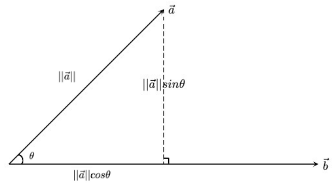
orthogonal projection of $\overrightarrow{a}$ onto $\overrightarrow{b}$ ($proj_{\overrightarrow{b}}\overrightarrow{a}$)

 

1. Magnitude of projection vector (component of projection)

   $||proj_{\overrightarrow{b}}\overrightarrow{a}|| = ||\overrightarrow{a}||cos\theta$

   In addition, realize that $\overrightarrow{a}\cdot\overrightarrow{b} = ||\overrightarrow{a}||||\overrightarrow{b}||cos\theta$

   $\frac{\overrightarrow{a}\cdot\overrightarrow{b}}{||\overrightarrow{b}||} = ||\overrightarrow{a}||cos\theta$

   $||proj_{\overrightarrow{b}}\overrightarrow{a}|| = \frac{\overrightarrow{a}\cdot\overrightarrow{b}}{||\overrightarrow{b}||}$

2. Projection vector (unit vector in direction of $\overrightarrow{b}$ scaled by component)

   $proj_{\overrightarrow{b}}\overrightarrow{a} = (\frac{\overrightarrow{a}\cdot\overrightarrow{b}}{||\overrightarrow{b}||}) \frac{\overrightarrow{b}}{||\overrightarrow{b}||} = (\frac{\overrightarrow{a}\cdot\overrightarrow{b}}{||\overrightarrow{b}||^2})\overrightarrow{b}$

Projection into Subspaces:

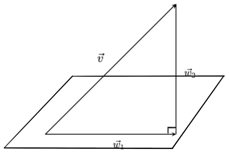
Let V be a vector space with subspace w, $\overrightarrow{w}, \overrightarrow{v}\in \overrightarrow{v}$

Theroem: If V is a vector space and W is a subspace of V then for each $\overrightarrow{v} \in V$

$\overrightarrow{v} =\overrightarrow{w}_1 + \overrightarrow{w}_2$ where $\overrightarrow{w}_1\in W$ and $\overrightarrow{w}_2\perp W$

How to determine $\overrightarrow{w}_1$ and $\overrightarrow{w}_2$?

Theorem: Let W be a finite dimensional subspace of a vector space V. If {$\overrightarrow{u}_1$,…, $\overrightarrow{u}_n$} is an orthonormal basis of W and $\overrightarrow{x} \in V$ then $proj_{W}\overrightarrow{x} = \frac{\overrightarrow{x} \cdot \overrightarrow{v}_1}{||\overrightarrow{v}_1||^2}\overrightarrow{v}_1 + ...+ \frac{\overrightarrow{x} \cdot \overrightarrow{v}_n}{||\overrightarrow{v}_n||^2}\overrightarrow{v}_n$

Example:

Let $V = \mathbb{R}^3$ and $W =$ span{$\begin{bmatrix} 0 \\ 1 \\ 0 \\ \end{bmatrix}$, $\begin{bmatrix} -\frac{4}{5} \\ 0 \\ \frac{3}{5} \\ \end{bmatrix}$}. Compute $proj_{W}\overrightarrow{x}$ where $\overrightarrow{x} = <1,1,1>$

$\therefore proj_{W}\overrightarrow{x} = (<1,1,1>\cdot <0,1,0>) \begin{bmatrix} 0 \\ 1 \\ 0 \\ \end{bmatrix} + (<1,1,1> \cdot <-\frac{4}{5},0,\frac{3}{5}>)\begin{bmatrix} -\frac4{5} \\ 0 \\ \frac{3}{5} \\ \end{bmatrix} = \begin{bmatrix} 0 \\ 1 \\ 0 \\ \end{bmatrix} + \begin{bmatrix} \frac{4}{25} \\ 0 \\ -\frac{3}{25} \\ \end{bmatrix} = \begin{bmatrix} \frac{4}{25} \\ 1 \\ -\frac{3}{25} \\ \end{bmatrix}$

$proj_{W}\overrightarrow{x} = \overrightarrow{w}_1$

$\therefore \overrightarrow{w}_2 = \overrightarrow{x} - proj_{W}\overrightarrow{x} = \begin{bmatrix} \frac{21}{25} \\ 0 \\ \frac{28}{25} \\ \end{bmatrix}$

Key Result

Theorem: Every finite dimensional vector space has an orthonormal basis.

Proof: We will proceed by constructing an algorithmic solution:

The Gram-Schmidt Process:

*Goal: Given a basis of a vector space construct an orthonormal basis.

Let {$\overrightarrow{u}_1$,…, $\overrightarrow{u}_n$} be any basis and {$\overrightarrow{v}_1$,…, $\overrightarrow{v}_n$} be the desired orthonormal basis.

1. $\overrightarrow{v}_1 = \overrightarrow{u}_1$

2. Let $\overrightarrow{w}_1 =$ span{$\overrightarrow{v}_1$}

   $\therefore \overrightarrow{v}_2 = \overrightarrow{u}_2 - proj_{w_1}\overrightarrow{u}_2$

   $\therefore \overrightarrow{v}_2 = \overrightarrow{u}_2 - \frac{\overrightarrow{u}_2 \cdot \overrightarrow{v}_1}{||\overrightarrow{v}_1||^2}\overrightarrow{v}_1$

3. Let $\overrightarrow{w}_2 =$ span{$\overrightarrow{v}_1$, $\overrightarrow{v}_2$}

   $\therefore \overrightarrow{v}_3 = \overrightarrow{u}_3 - proj_{w_2}\overrightarrow{u}_3$

   $\therefore \overrightarrow{v}_3 = \overrightarrow{u}_3 - \frac{\overrightarrow{u}_3 \cdot \overrightarrow{v}_1}{||\overrightarrow{v}_1||^2}\overrightarrow{v}_1 - \frac{\overrightarrow{u}_3 \cdot \overrightarrow{v}_2}{||\overrightarrow{v}_2||^2}\overrightarrow{v}_2$

…

Continue in this fashion up to $\overrightarrow{v}_n$

Example:

Use the Gram-Schmidt process to transform the basis $\overrightarrow{u}_1 = <1,1,1>$, $\overrightarrow{u}_2 = <0,1,1>$, $\overrightarrow{u}_3 = <0,0,1>$

1. $\overrightarrow{v}_1 = \overrightarrow{u}_1 = <1,1,1>$

2. $\overrightarrow{v}_2 = \overrightarrow{u}_2 - proj_{\overrightarrow{w_1}}\overrightarrow{u}_2$

   $\overrightarrow{v}_2 = <0,1,1> - \frac{\overrightarrow{u}_2 \cdot \overrightarrow{v}_1}{||\overrightarrow{v}_1||^2}\overrightarrow{v}_1$

   $\overrightarrow{v}_2 = <0,1,1> - \frac{2}{3}<1,1,1>$

   $\overrightarrow{v}_2 = <0,1,1> - <\frac{2}{3},\frac{2}{3},\frac{2}{3}>$

   $\overrightarrow{v}_2 = <-\frac{2}{3},\frac{1}{3},\frac{1}{3}>$

3. $\overrightarrow{v}_3 = \overrightarrow{u}_3 - proj_{w_2}\overrightarrow{u}_3$

   $\overrightarrow{v}_3 = \overrightarrow{u}_3 - \frac{\overrightarrow{u}_3 \cdot \overrightarrow{v}_1}{||\overrightarrow{v}_1||^2}\overrightarrow{v}_1 - \frac{\overrightarrow{u}_3 \cdot \overrightarrow{v}_2}{||\overrightarrow{v}_2||^2}\overrightarrow{v}_2$

   $\overrightarrow{v}_3 = <0,0,1> - \frac{1}{3}<1,1,1> - \frac{1}{2}<-\frac{2}{3},\frac{1}{3},\frac{1}{3}>$

   $\overrightarrow{v}_3 = <0,-\frac{1}{2},\frac{1}{2}>$

   $\therefore \overrightarrow{v}_1, \overrightarrow{v}_2, \overrightarrow{v}_3$ orthogonal (not orthonormal)

4. Normalize => unit vectors

   $\overrightarrow{v}_1$ => $\frac{1}{||\overrightarrow{v}_1||}\overrightarrow{v}_1 = <\frac{1}{\sqrt{3}},\frac{1}{\sqrt{3}},\frac{1}{\sqrt{3}}>$ Repeat for $\overrightarrow{v}_2$,$\overrightarrow{v}_3$

2.5 Labs

Fields Lab (2.1: Vector Spaces)

Chemical Balancing Lab (2.2: Linear Independence, Basis, and Dimension)

2.6 Coding Labs

Dimensional Analysis (2.2: Linear Independence, Basis, and Dimension)

2.6.1 Orthogonality, Gram-Schmidt Process, and SVD (2.4-2.5: Projects & Fundamental Theorem of Linear Algebra)

2.6.2 Coding Key