
Chapter 8 Data Wrangling
8.1 Intro
Data Wrangling is the process of cleaning and manipulating your data.frame. I have never obtained a dataset that did not need to be cleaned or organized in some fashion (if you have I am quite jealous). The packages I rely on the most are
- tidyverse (specifically dplyr & tidyr)
- janitor
- hablar
My suggestion is to take this cheat sheet and frame it. Over time you will become VERY familiar with these functions but you can’t expect that of yourself this early. Although the cheat sheet goes through many of the functions you will need, I will go through a few common tasks below.
If you want to learn more on why Data Wrangling is so important check out Hadley Wickham’s paper here it provides a thorough breakdown of its importance.
8.2 Tasks
8.2.1 Inspecting the imported data
Among the issues you may encounter with your data is inconsistencies in columnnames. This can be rather annoying. In order to alleviate this, I like to pick one format and stick with it. When I receive a dataset from another researcher I will often use snakecase to modify their dataset accordingly. This package is incorporated into janitor
If you want to check for missing cases you can use the following code
sapply(df, function(x) sum(is.na(x)))8.2.2 Choosing good column names
- Avoid using spaces. This makes it more tedious to refer or call a column later on. In the example below our task is to rename the column “Group Level”. It should also be noted that things can get tricky when you are using certain packages and will over time, be a large burden to you. Hence, my advice is to remove spaces. Consider going into snakecase.
df$`Group Level` # Column name with spaces

df$GroupLevel # Column name without spaces
Because of this, one of my first steps is to use clean_names() from the janitor package. It will
- Parses letter cases and separators to a consistent format.
- Default is to snake_case, but other cases like camelCase are available
- Handles special characters and spaces, including transliterating characters like œ to oe.
- Appends numbers to duplicated names
- Converts “%” to “percent” and “#” to “number” to retain meaning
- Spacing (or lack thereof) around numbers is preserved
df <- import("raw/dirty-data.xlsx", which = 2) # import a dataset with dirty column names

df %>%
    janitor::clean_names()
There are a few ways to rename your variables. The key is to pick your favorite and stick to it. My recommendation while coding is to avoid using spaces if at all possible, they will make your life miserable. Below are a few examples you can consider.
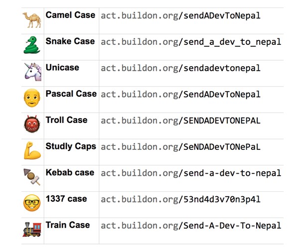
Figure 8.1: CamelCase source:https://targetstudy.com/nature/animals/camel.html

Figure 8.2: Naming Convention Styles
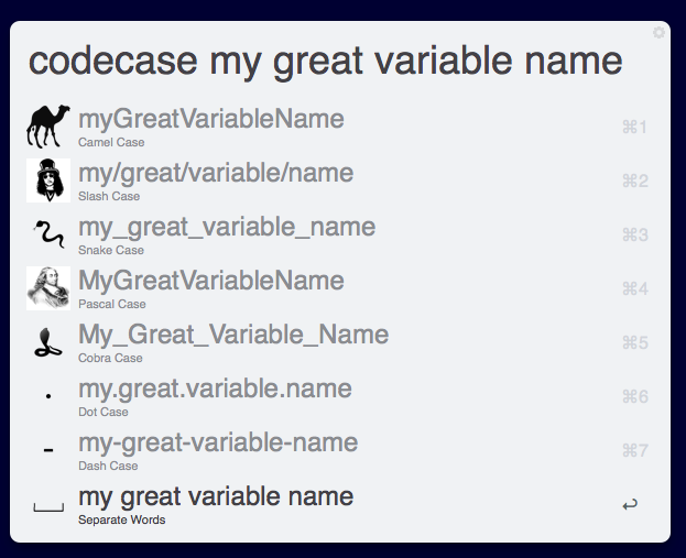
Figure 8.3: Naming Convention Styles 2
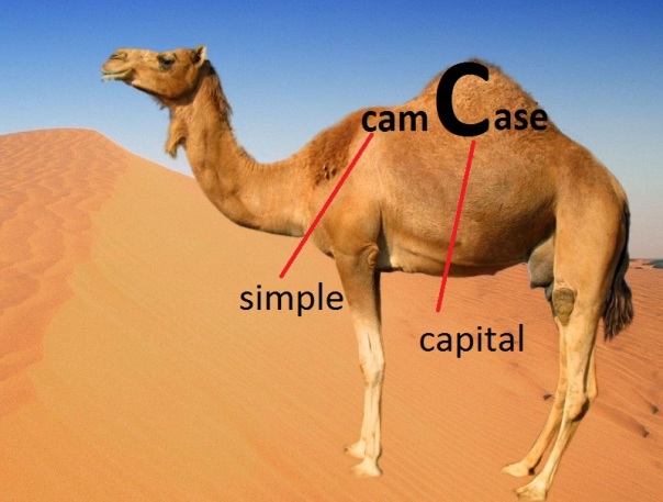
Figure 8.4: CamelCase source:https://targetstudy.com/nature/animals/camel.html
You can take a deep dive into some naming convention options by reading about the snake_case package documentation. I would recommend the breakdown by Almost Random
You can also view a presentation from the UseR Conference in 2017 here

8.2.3 Filtering data
Filtering your data is arguably the most common task you will repeat. There are several ways to filter data. The code chunk below goes through a few examples
# Filtering based on a partial string match
mtcars %>%
        filter(str_detect(rowname, "Merc")) # this will filter everything that has the pattern "Merc" in the column

# Removing a column based on a string match
df <- filter(df, C != "Foo") # filter any column that is not equal to "Foo"
8.2.4 Rounding columns
This will come in handy when we create tables to be used in our Rmd document In some instances you might want to round all numeric columns.
df %>%
mutate(across(where(is.numeric), round, 1)) # round to 1 decimal point
However, in most of my own datasets I do not want to round across all columns.
# Method #1
df %>%
 mutate(across(c(vnum1, vnum2), ~ round(., 1))) # where "vnum1" and "vnum2" are column names

# Method #2
df %>%
   janitor::adorn_rounding(digits =2)
8.2.5 Selecting columns
Very useful in case you want to remove specific columns
# Example 1
df <- df %>%
select(-c("column1", "column2")) # This will remove "column1" and "column2" from df

# Example 2
tmp <- md.df %>%
            dplyr::select(metric:Right_UF)
8.2.6 Removing Blanks
Below are a few different ways to removes blanks, which are imported as NA in RStudio data.frames
# Method 1 - dplyr
df <- df %>%
      filter(!is.na(columnName)) # give me a new dataframe with only the international services.

# Method #2 - janitor
df <- df %>%
      janitor::remove_empty(c("rows", "cols") # remove all blank rows and columns
8.2.7 Creating factors
These come in handy when we want to run statistics and/or when you want a specific order when plotting
df$intrahemispheric_nirs <- factor(df$intrahemispheric_nirs, ordered = TRUE, levels = c("No", "Yes", exclude=""))8.2.8 Renaming a column
df <- df    %>%
    dplyr::rename(
      #‘New Column Name’= ‘Old Name’
      "month"= "Month"
    )
8.2.9 Replace strings using pipes
In the code below I want to replace text in the Test column. Notice how I call the column once and then use the pipe operator to list the rest
df %>%
mutate(Test = str_replace_all(Test, ":", "×") %>%
         str_replace_all("group2.L", "Group") %>%
         str_replace_all("mriloc2", "") %>%
         str_replace_all("hemisphereLeft", "LeftHemi") %>%
         str_replace_all("hemisphereRight", "RightHemi")
)
8.2.10 Add column in specific spot
df <- add_column(df, "DMT_line2" = df$DMT_line, .after = "DMT_line")

# Add a blank column in a specific spot =====
  items <- add_column(items, "Avg" = replicate(length(items$value.D1), NA) , .after = "value.D7")
8.2.11 Create new columns based on conditions (Advanced)
We won’t go into this in much detail for now but you can also choose to mutate based on conditions using case_when which has come up very useful for me in the past.
8.2.11.1 Example 1
 # Example #1

 d <- d %>%
        mutate(a_sportinj= case_when( (is.na(new_moic3q2a) == TRUE & new_moic3q2 == "Non-sport related injury") ~ 'Non-Sport',
                                      new_moic3q2a == "Sports" ~ 'Sport',
                                      new_moic3q2a == "Recreation Activity (not sport)" ~ 'Recreation',
                                      (new_moic3q2a == "Unknown (cannot be determine from the information given)" | is.na(new_moic3q2a) == TRUE) & new_moic3q2 == "Non-sport related injury" ~ 'Non-Sport')
        )
8.2.12 Example 2
# Example #2
df.nirs <- df.nirs %>%
                dplyr::mutate(MRI_Completed = case_when((df.nirs$Subject %in% ids == "TRUE") ~ 'Yes',
                                                 (df.nirs$Subject %in% ids == "FALSE") ~ 'No'))
8.2.13 Example 3
# Example #3

df.mix <- df.mix %>%
      mutate(
        intrahemispheric_nirs= case_when(
          Connection == "L-DLPFC->R-DLPFC" ~ 'Yes',
          Connection == "L-DLPFC->R-Motor" ~ 'Yes',
          Connection == "R-DLPFC->L-Motor" ~ 'Yes',
          Connection == "L-Motor->R-Motor" ~ 'Yes',
          Connection == "L-DLPFC->L-Motor" ~ 'No',
          Connection == "R-DLPFC->R-Motor" ~ 'No')) # Is the NIRS S-D intrahemispheric?
8.3 Converting from wide to long
Almost without exception, you will want your data to be in the “long” format. This can be a tricky operation.

Figure 8.5: Long vs Wide dataframes
Almost without exception, you will want your data to be in the “long” format. There are several papers which explain why this is the preferred practice.

Figure 8.6: Long vs Wide dataframes
8.4 Merging dataframes
This is a very common task for example, in my experiments it’s common to have 2 files
- Neuroimaging data
- Demographic data
There are several ways to “join” dataframes. We want to “merge” these into one big data.frame….how do we do it???

Figure 8.7: My experience with MATLAB plots
First, we need to see which columns the datasets have in common and confirm the columns are named the same.
df <- import("raw/data.xlsx", which = "anova-data")
df.demo <- import("raw/data.xlsx", which = "demographics") %>% # Imports the sheet with demographic data
  janitor::clean_names() # Clean the column names
As we inspect the data we see that in df the column ID is named study_id in df.demo. Similarly Group in df is named group in df.demo. We can save ourselves some headaches by adding a few lines after importing the data.
df <- import("raw/data.xlsx", which = "anova-data")
df.demo <- import("raw/data.xlsx", which = "demographics") %>% # Imports the sheet with demographic data
  janitor::clean_names() %>% # Clean the column names
  dplyr::rename(
  # New Name = Old Name
    "ID" = "study_id",
    "Group" = "group"
  )
Now we can finally merge the columns. We want to merge by ID. There are several ways to join data. In our example we are going to use left_join. Within the function, two dataframes are called (usually referred to as x and y). In the animation below “x” is df while “y” is df.demo.
Figure 8.8: left_join
tmp <- left_join(df, df.demo, by = "ID") Notice that at the moment, we have two Group columns. One coming from the x dataframe which is df and one stemming from the y dataframe df.demo. In order to fix this problem we are going to add another column to join in our statement
tmp <- left_join(df, df.demo, by = c("ID", "Group")) We now have a dataset which has both the concussion score and demographic data combined into one! Before continuing I like to remove dataframes that are no longer in use. This keeps our Global Environment tidy.
df <- tmp           # name the combined dataframe "df"
rm(tmp, df.demo)    # remove the datasets that we don't need
8.4.1 Exercises
For students looking to get more practice on merging datasets, I would highly recommend the Relational Data chapter of the R for Data Science book by Garrett Grolemund and Hadley Wickham.
8.4.2 Drew’s Notes
- This is a great breakdown
- There is an animation on GitHub I should probably copy to explain the difference
- Animations
8.4.3 Supplementary Resources
Here are a few resources on wide vs long data formats
Below is a list of pages I have collected that have come in very useful for beginners
8.4.3.1 Selecting using the tidyverse
8.4.3.2 Working with dates
We won’t cover working with dates much in this guide, because its not typical. However, should you need them the link below provides a general walkthrough.
8.4.4 Misc Code
Misc code is shown below. This is for me, while I finish the book. Please ignore it for now.
# Adding Names to Columns ==================
# This can be required when using certain plotting functions like "likert" --> see ALPH likert4.R
names(items) <- c(
  symptoms_decLOC="Did the patient have loss of consciousness?",
  symptoms_headache="Did the patient have headaches?",
  symptoms_nausea_vomitting="Did the patient have nausea/vomiting?",
  symptoms_cranialNerve_paresis="Did the patient have cranial nerve paresis?",
  symptoms_gait_disturbance="Did the patient have any gait disturbances?")
# Data Wrangling ----------------
df1$Group <- rep("Body", length(df1$`File name`))
df2$Group <- rep("Genu", length(df2$`File name`))
df3$Group <- rep("Splenium", length(df3$`File name`))

idx <- unique(df3l$`File name`) == df1$`File name`

dfx <- df1 %>%
  select_if(df1$`File name` == unique(df3$`File name`))
combinedDF <- rbind(df1,df2,df3)

df1[!(df1$`File name` %in% df3$`File name`)]

idx <- setdiff(df1$`File name`, df2$`File name`)
df1 <- df1[,idx]

# Convert several columns to numeric ----------
 cols <- grep(pattern = "CC_F|Left|Right", x = names(df), value = TRUE)
 df[, cols] <- lapply(df[ , cols], function(x) suppressWarnings(as.numeric(x))) #supressWarnings is so you don't get "NAs introduced by coercion" in your console output
# Count the number of NA's in each column of a dataframe ----------
sapply(df, function(x) sum(is.na(x))) #this is different than "summary(df)" which gives you information on more than NA's

# Add column in specific spot ========
df <- add_column(df, "DMT_line2" = df$DMT_line, .after = "DMT_line")

# Add a blank column in a specific spot =====
  items <- add_column(items, "Avg" = replicate(length(items$value.D1), NA) , .after = "value.D7")

# Remove blank rows in a specific column =======
df <- df[-which(df$start_pc == ""), ]

# Removing a column based on a string match =========
        df <- filter(df, C != "Foo")
  # Renaming a variable in a column : str_replace (this won't take exact strings)=============
  df1$ID <- df$ID   %>%
    str_replace("pi6437934_2", "S2")

  # Replace an exact string -------------
  data$OpenBCI_FileName <- gsub("\\<y\\>","", data$OpenBCI_FileName) # replaces cols with "y" but won't touch something like "My Drive"

  # if you have multiple strings to replace you can use the pipe operator to get everything done in one shot
  df$ID <- df$ID    %>%
    str_replace("pi_14344894_9", "S9") %>% #oldstring, newstring
      str_replace("pi_3478_03o4_15", "S15")

  # Partial String match in a column----------
    # __Method 1: str_detect ========
      mtcars %>%
        filter(str_detect(rowname, "Merc")) # this will filter everything that has the pattern "Merc" in the column

    # __Method 2 : grepl ==========
    dplyr::filter(mtcars, !grepl('Toyota|Mazda', type)) # Using grepl
    cols <- grep(pattern = "symptoms|Previous_shunt", x = names(df), value = TRUE) #Select columns that start with symptoms
    df[cols] <- as.data.frame(lapply(df[cols],function(x) {factor(x,levels=mylevels, exclude="")}))

    #__Method 3 : grep (similar to grepl) =====
    cols <- grep(pattern = "symptoms", x = names(df2), value = TRUE) #Select columns that start with symptoms


  # Renaming a column ================
  df <- df  %>%
  df <- df  %>%
    dplyr::rename(
      #‘New Column Name’= ‘Old Name’
      "month"= "Month"
    )

  # Removing NA's-----------
    # __Method 1: is.na() ====
    df <- df %>%
      filter(!is.na(columnName)) # give me a new dataframe with only the international services.

    # __Method 2: na.omit() ====
    df1 <- na.omit(df1)

  # Filtering our data that fits a condition: filter=========
  new_df <- filter(df, service=="International") # give me a new dataframe with only the international services.
To rename parts of a column using %>% you need to use mutate
# normal way to replace strings in a column
df$columnName = str_replace_all(df$columnName, "Contribution_", "")

# Using pipe
df %>%
mutate(columnName = str_replace_all(columnName, "Contribution_", ""))

# Be careful when special characters are involved. You will need to add a "break"
df <- df %>%
  mutate(Age = str_replace_all(Age, "All ages \\(15 to 74 years\\)", "Test"))

# If you use the following code, it will not work
df <- df %>%
  mutate(Age = str_replace_all(Age, "All ages (15 to 74 years)", "Test"))
You can also choose to mutate based on conditions using case_when which has come up very useful for me in the past.
 d <- d %>%
        mutate(a_sportinj= case_when( (is.na(new_moic3q2a) == TRUE & new_moic3q2 == "Non-sport related injury") ~ 'Non-Sport',
                                      new_moic3q2a == "Sports" ~ 'Sport',
                                      new_moic3q2a == "Recreation Activity (not sport)" ~ 'Recreation',
                                      (new_moic3q2a == "Unknown (cannot be determine from the information given)" | is.na(new_moic3q2a) == TRUE) & new_moic3q2 == "Non-sport related injury" ~ 'Non-Sport')
        )
8.5 For Item-based data
The likert package seems great. I have used it to great success in past projects.
8.5.1 Suggested Reading
- Why you should use pipes
- Data Manipulation with dplyr
- Column-wise operations using dplyr
- Article by the New York Times
8.5.2 Links for Andrew
- Presentation on Data Wrangling
- Chapter on Data Wrangling
- Another Chapter
- This site has a bunch of exercises that might be useful for the workshop.
- This package might be a good GUI for beginners but I need to test it first.