Chapter 8 Advanced options

8.1 Custom regional summaries

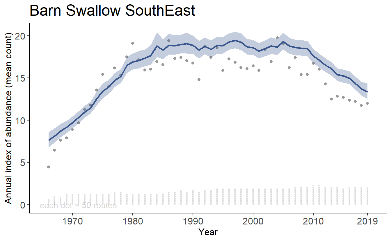
Yes, you can calculate the trend and trajectories for custom combinations of strata, such as a formal trend estimate for populations of Barn Swallow in the South East portion of their range (e.g., BCRs 21,24,25,26,27,35,36, and 37).

8.1.1 Define the custom regions as a collection of the existing strata.

First extract a dataframe that defines the original strata used in the analysis.

st_comp_regions <- get_composite_regions(strata_type = "bbs_cws")
knitr::kable(head(st_comp_regions))

prov_state	region	area_sq_km	national	bcr	Province_State	Country	bcr_by_country
AB	CA-AB-10	52565	CA	10	Alberta	Canada	Canada-BCR_10
AB	CA-AB-6	445136	CA	6	Alberta	Canada	Canada-BCR_6
AB	CA-AB-8	6987	CA	8	Alberta	Canada	Canada-BCR_8
AB	CA-AB-11	149352	CA	11	Alberta	Canada	Canada-BCR_11
AK	US-AK-1	9551	US	1	ALASKA	United States of America	United States of America-BCR_1
AK	US-AK-2	283405	US	2	ALASKA	United States of America	United States of America-BCR_2

Then add a column to the dataframe that groups the original strata into the desired custom regions.

st_comp_regions$SouthEast <- ifelse(st_comp_regions$bcr %in% c(21,24:27,35:37),"SouthEast","Other")

8.1.2 Use defined regions to estimate indices and trends

st_comp_regions can now be used as the dataframe input to the argument alt_region_names in generate_indices(), with “SouthEast” as the value for the argument regions. The relevant trends can be calculated using just the generate_trends() function.

library(patchwork)
custom_indices <- generate_indices(jags_mod = jags_mod,
                                      jags_data = jags_data,
                                      alt_region_names = st_comp_regions,
                                      regions = "SouthEast")
tp = plot_indices(indices = custom_indices,
                         species = "Barn Swallow",
                  add_observed_means = TRUE,
                  add_number_routes = TRUE,
  title_size = 20,
  axis_title_size = 12,
  axis_text_size = 12)

print(tp[[1]])
print(tp[[2]])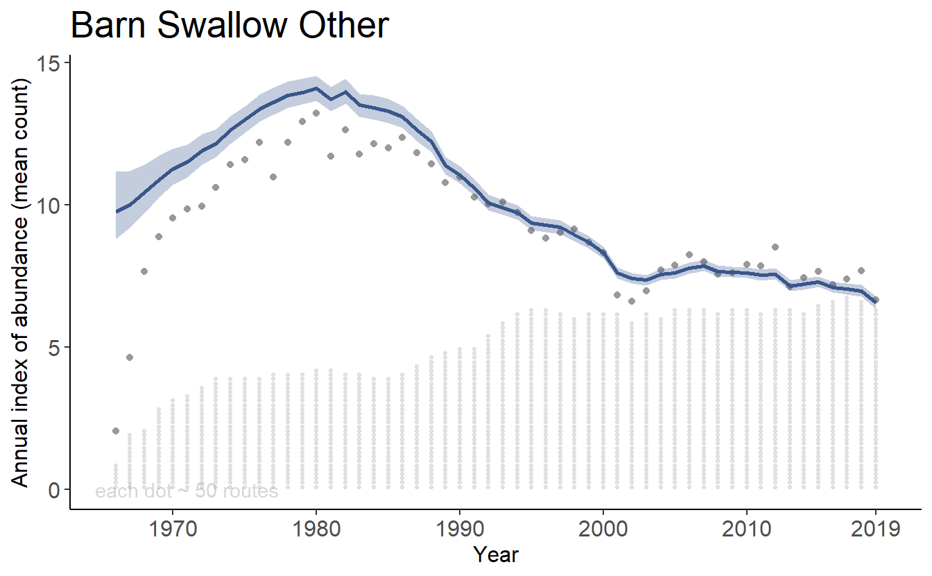

Calculate trends

custom_trends <- generate_trends(indices = custom_indices)
knitr::kable(custom_trends[,c(1,3,8,9,14)])

8.2 Exporting the JAGS model

You can easily export any of the bbsBayes models to a text file.

model_to_file(model = "slope",
              filename = "my_slope_model.txt")

This is the best way to confirm all of the priors, and model structures.

8.3 Customizing the JAGS model and data

You can also modify the model text (e.g., try a different prior) and run the modified model

run_model <- function(... ,
                      model_file_path = "my_modified_slope_model.txt",
                      ... )

Or, you could add covariates. For example a GAM smooth to estimate the effect of the day of year on the observations, or an annual weather covariate, or… Then add the relevant covariate data to the jags_data object, and you’re off!

Here’s a GitHub repo with an example of a modified bbsBayes model. The modified model includes a series of GAM smooths to account for variation in counts over the course of the BBS observation season (mid-May through early July). In addition these seasonal smooths are allowed to vary by decade to account for possible shifts in phenology through time.

https://github.com/AdamCSmithCWS/BBS_seasonal_shift_ALHU

8.4 Comparing Models

Finally, bbsBayes can be used to run cross-validations. For example, the get_final_values() function is useful to provide an efficient starting point for a cross-validation runs, without having to wait for another full burn-in period.

Paper that includes an example of how to implement a cross-validation using bbsBayes.

Ornithological Applications: https://doi.org/10.1093/ornithapp/duaa065 Supplement: https://zenodo.org/badge/latestdoi/228419725

NOTE: although bbsBayes includes functions to calculate WAIC, recent work has shown that WAIC performs very poorly with the BBS data (https://doi.org/10.1650/CONDOR-17-1.1). We recommend a k-fold cross-validation approach, as in the above zenodo archive.