Chapter 1 What is statistical power?

Statistical power is a factor that helps determine how likely our study is to achieve its goals. You may recall learning about Type I and Type II Errors in Topic 5. To recap, we can summarise these types of errors as follows:

There are two types of error that can occur:

Type I error: Reject \(H_0\) when \(H_0\) is true.
Type II error: Fail to reject \(H_0\) when \(H_0\) is false.

Another way to think about Type I and Type II errors is via the following table:

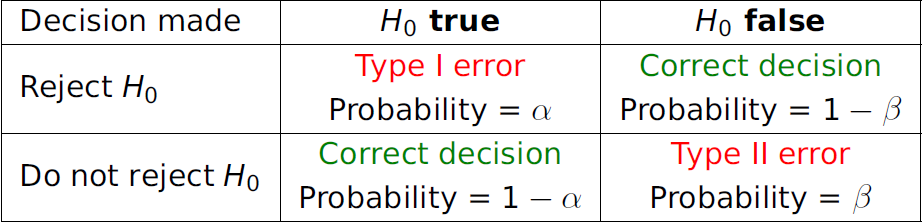
As we know, a Type I error occurs when we reject \(H_0\) when \(H_0\) was actually true, and the probability of this occurring is equal to the significance level \(\alpha\). On the other hand, a Type II error occurs when we fail to reject \(H_0\) when \(H_0\) was actually false. We can denote the probability of this occurring as \(\beta\). As it turns out, statistical power is the opposite of a Type II error:

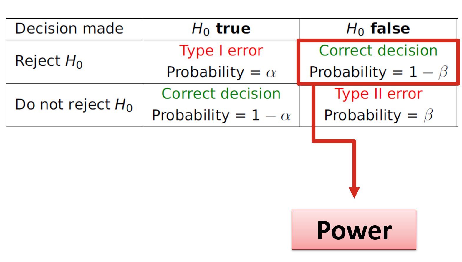
That is, power is the probability of making the correct decision to reject \(H_0\) given that \(H_0\) is actually false. One way to understand statistical power would be to think of it like this:

What is statistical power?

Statistical power is the probability of actually getting a significant result when it is truly there to be found.

Holding all other things equal, increasing the sample size will increase power, whereas decreasing the sample size will decrease power. By the same token, increasing the sample size will increase the cost of the study in most cases, and often with diminishing returns once a certain level of power is reached. Just like the significance level \(\alpha\), which is typically chosen to be 0.05, a typical level of statistical power to aim for is 0.8 (or 0.9). That is, sample sizes are often chosen such that, if \(H_0\) is false, the probability of rejecting \(H_0\) would be 0.8. We will see some examples in the next section.