Chapter 5 Intro to Regression

This section was originally prepared for the Adanced Methods of Political Analysis (Poli 706) in Spring 2019, which I served as a TA for Tobias Heinrich.

5.1 Why do we need a model?

To quote Hadley Wickham, “The goal of a model is to provide a simple low-dimensional summary of a dataset.” Ideally, a good model will capture the systematic patterns, while leaving out the “noises.” In social science, models are used for inference, i.e., confirming or rejecting that a hypothesis is true. See here for a different perspective from a data scientist. Before we proceed, please read the following quote.

“Now it would be very remarkable if any system existing in the real world could be exactly represented by any simple model. However, cunningly chosen parsimonious models often do provide remarkably useful approximations. For example, the law PV = RT relating pressure P, volume V and temperature T of an “ideal” gas via a constant R is not exactly true for any real gas, but it frequently provides a useful approximation and furthermore its structure is informative since it springs from a physical view of the behavior of gas molecules.

For such a model there is no need to ask the question “Is the model true?”. If “truth” is to be the “whole truth” the answer must be “No”. The only question of interest is “Is the model illuminating and useful?”"

— George Box

5.2 Model, prediction, and residuals

5.2.1 Prerequisite

In this section, we are going to need the following packages. Install them if you have not done so. The modelr package contains some simulated data that we are going to use for the sake of illustration. The tidyverse package is useful if you know tidy data and how to use pipes. If not, you can simply load ggplot2, which will suffice for this tutorial.

library(modelr)
library(tidyverse)
library(hexbin)

5.2.2 A simple regression

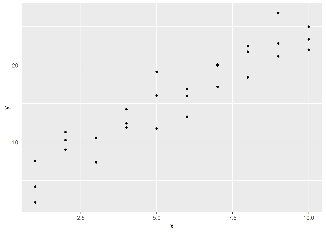
One of the simulated data sim1 contains two continuous variables x and y. Let’s take a look.

ggplot(sim1, aes(x, y)) + 
  geom_point()

From last semester, we know how to fit an OLS model.

sim1_mod <- lm(y ~ x, data = sim1)
summary(sim1_mod)

## 
## Call:
## lm(formula = y ~ x, data = sim1)
## 
## Residuals:
##     Min      1Q  Median      3Q     Max 
## -4.1469 -1.5197  0.1331  1.4670  4.6516 
## 
## Coefficients:
##             Estimate Std. Error t value Pr(>|t|)    
## (Intercept)   4.2208     0.8688   4.858 4.09e-05 ***
## x             2.0515     0.1400  14.651 1.17e-14 ***
## ---
## Signif. codes:  0 '***' 0.001 '**' 0.01 '*' 0.05 '.' 0.1 ' ' 1
## 
## Residual standard error: 2.203 on 28 degrees of freedom
## Multiple R-squared:  0.8846, Adjusted R-squared:  0.8805 
## F-statistic: 214.7 on 1 and 28 DF,  p-value: 1.173e-14

5.2.3 Predictions

Models make predictions. The OLS model we just fitted also makes predictions, which can be interpreted as the best guesses we can obtain under some assumptions. Let us predict the values of y using the OLS model.

grid <- data.frame(Intercept=1, x=seq_range(sim1$x, 10))
grid$pred <- predict(sim1_mod,grid)

Now let us plot the predicted line.

ggplot(sim1, aes(x)) +
  geom_point(aes(y = y)) +
  geom_line(aes(y = pred), data = grid, colour = "red", size = 1)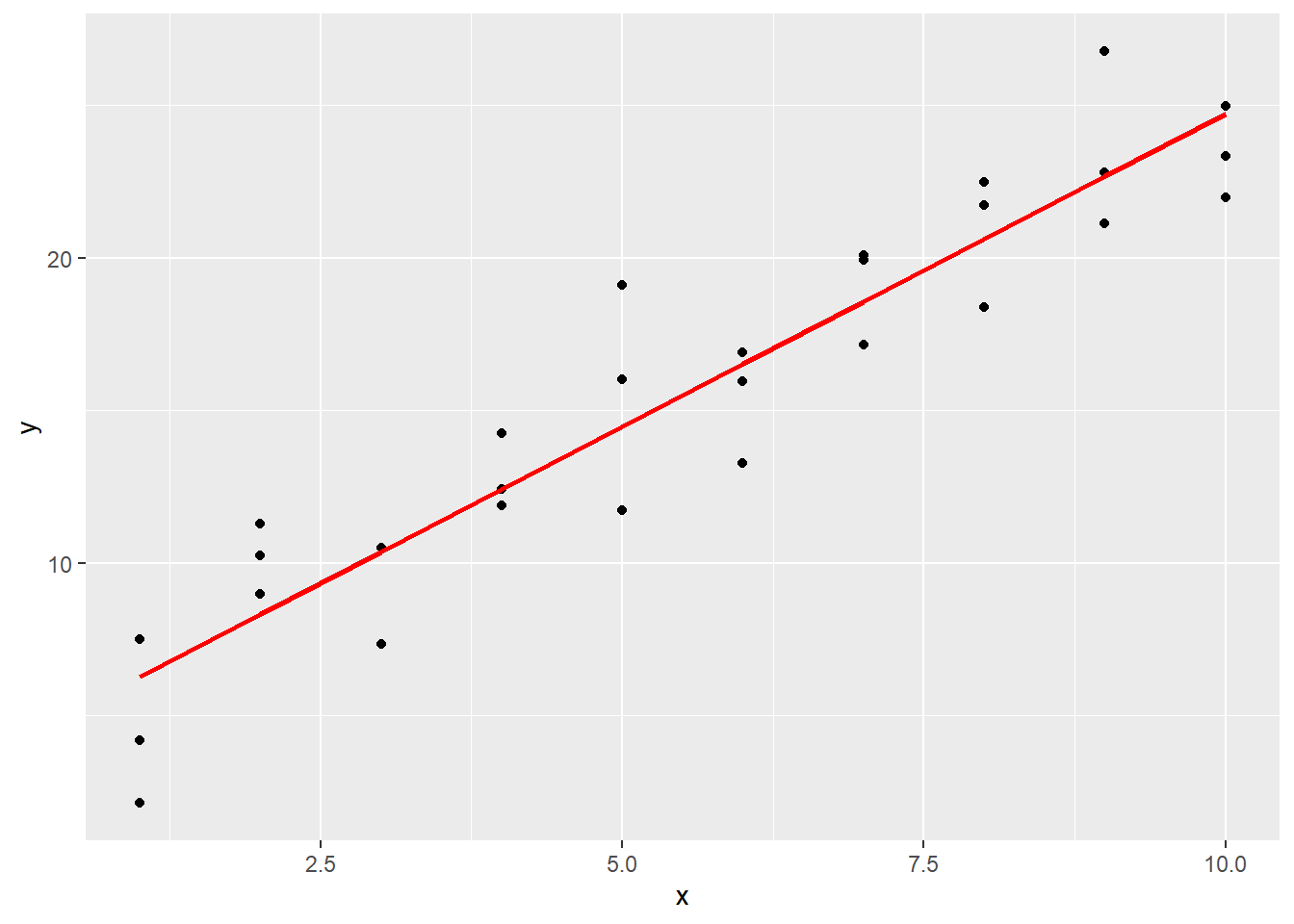

5.2.4 Residuals

Predictions tell us the pattern captured by the model, while residuals tell us the parts that the model missed. In essense, residuals are the difference between observed and predicted values. Let us plot the residuals of our OLS model.

sim1$resid <- residuals(sim1_mod)
ggplot(sim1, aes(x, resid)) + 
  geom_ref_line(h = 0) +
  geom_point()

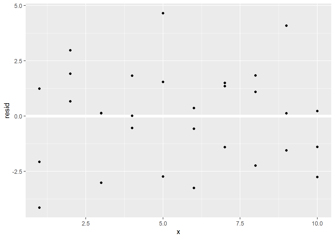
This looks like random noise. From what we have learned last semester, this indicates our OLS model appears to capture the systematic pattern and leaves out the “noises.”

5.3 A real world example: tacky diamonds are more expensive

Last semester we encountered the diamonds dataset from ggplot2. Let us plot the relationship between a diamond’s quality and its price.

ggplot(diamonds, aes(cut, price)) + geom_boxplot()

ggplot(diamonds, aes(color, price)) + geom_boxplot()

ggplot(diamonds, aes(clarity, price)) + geom_boxplot()

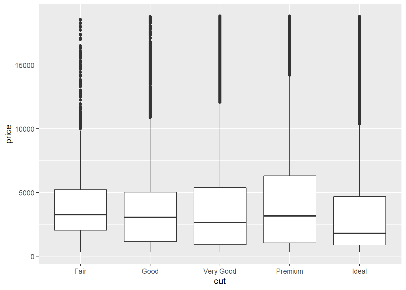
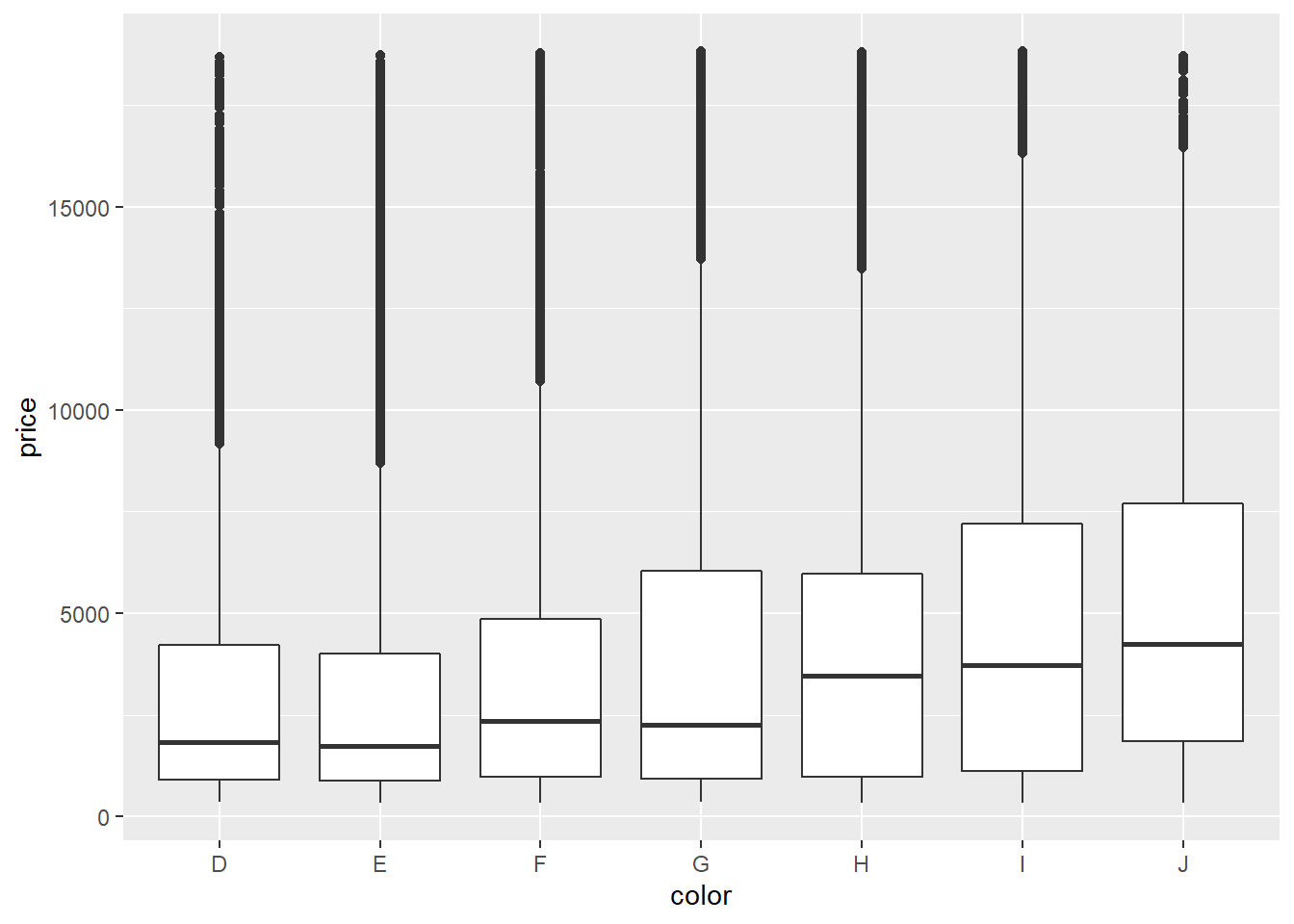
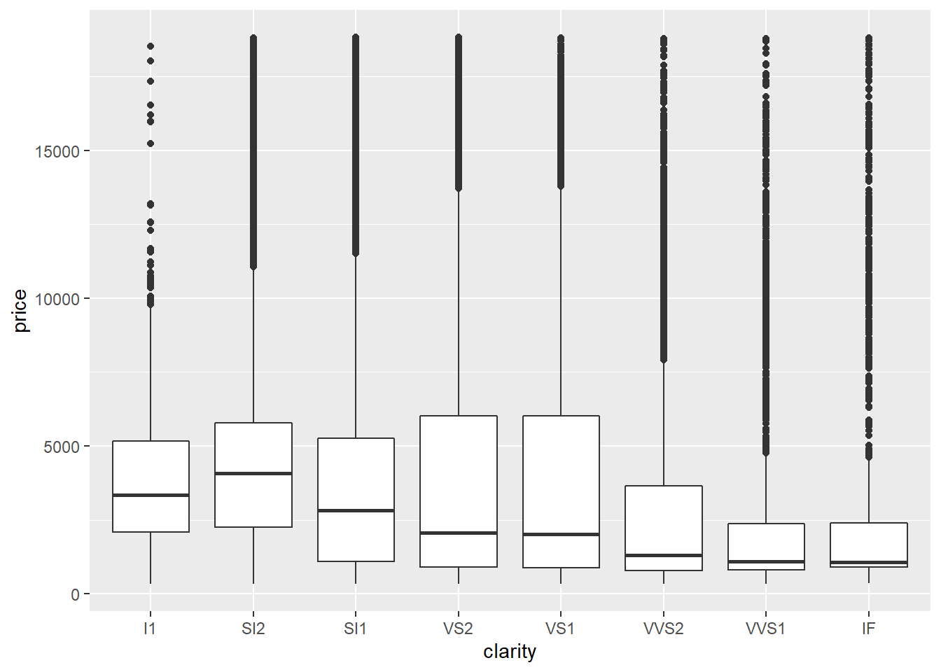
If we check the descriptions of the data (?diamonds), we know J is the worst color and I1 has the lowest clarity.

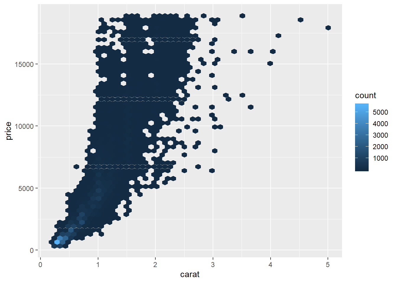
5.3.1 Confounding variable

The above results can be attributed to the fact that we are missing one important confounding variable: the weight of a diamond (carat). It could be the case that low-quality diamonds tend to be bigger.

carat_price_plot <- ggplot(diamonds, aes(carat, price)) + 
  geom_hex(bins = 50)
carat_price_plot

Now let us try modeling the relationship using OLS.

mod_diamond <- lm(price ~ carat, data = diamonds)

Add the predictions.

grid_diamond <- data.frame(Intercept=1, carat=seq_range(diamonds$carat, 10))
grid_diamond$price <- predict(mod_diamond,grid_diamond)
carat_price_plot + geom_line(data=grid_diamond, color="red", size=1)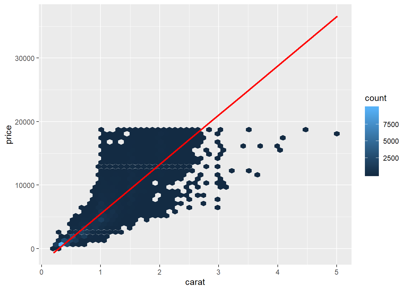

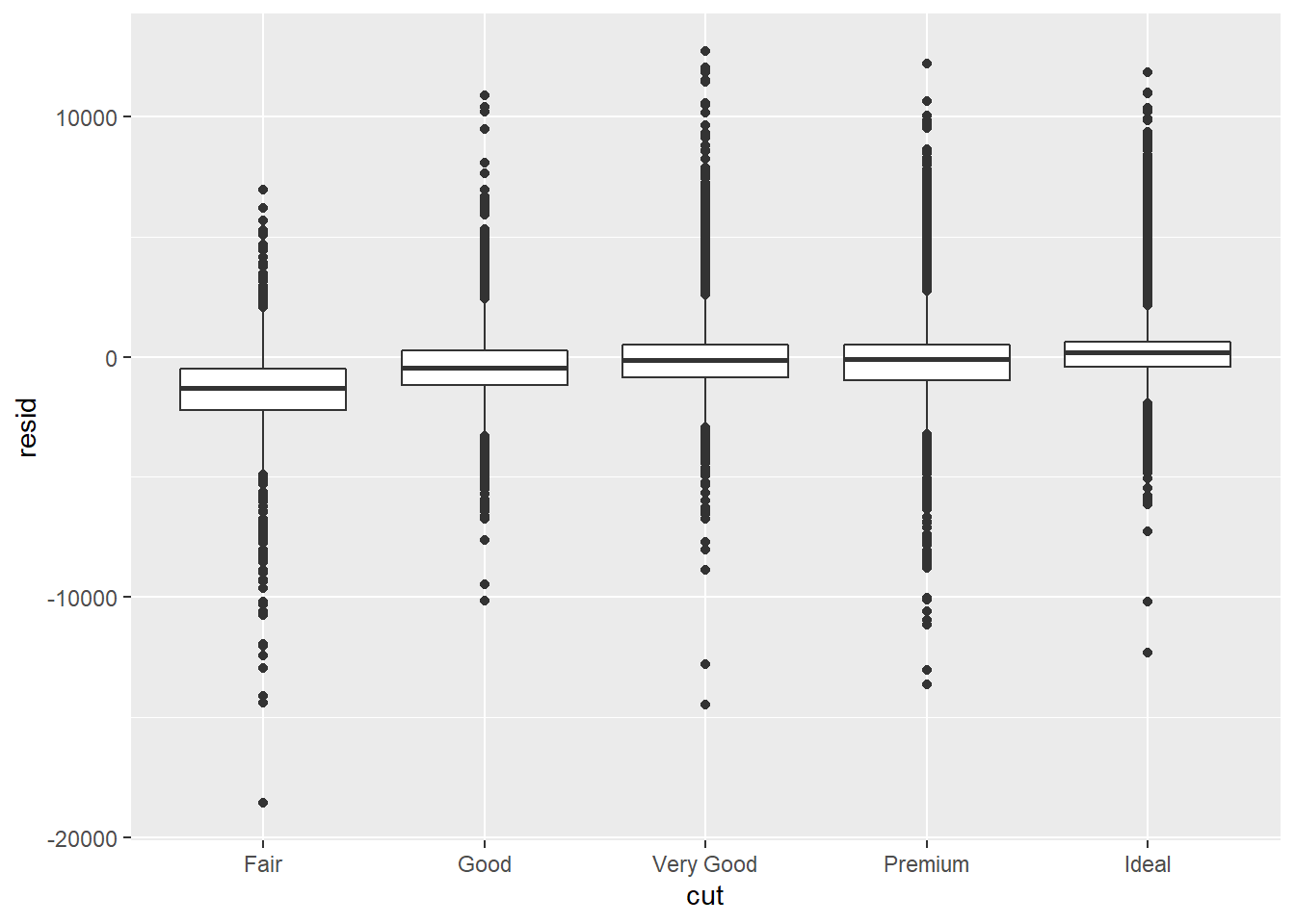
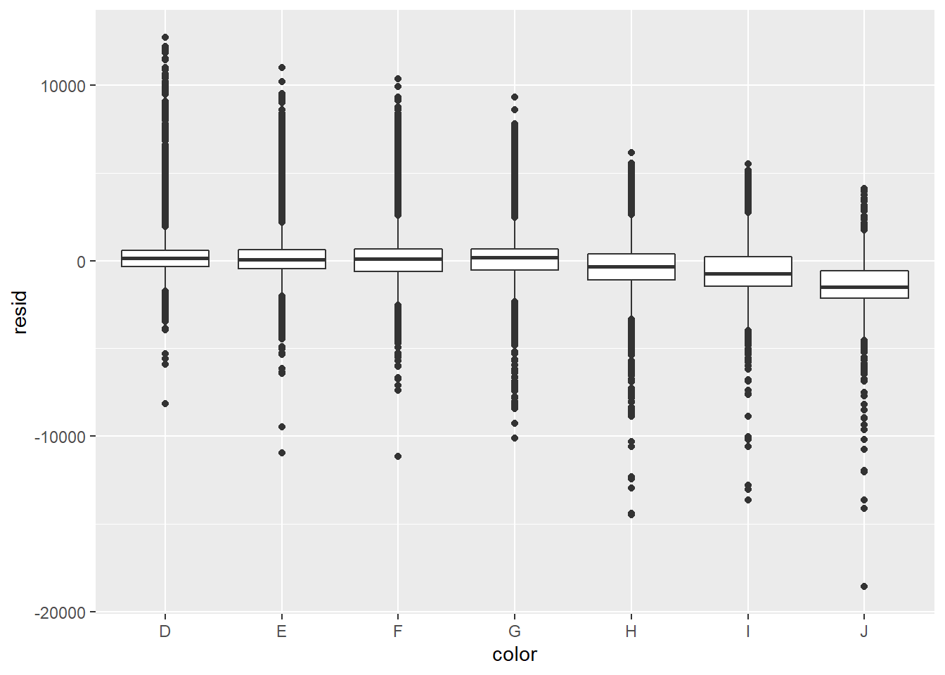
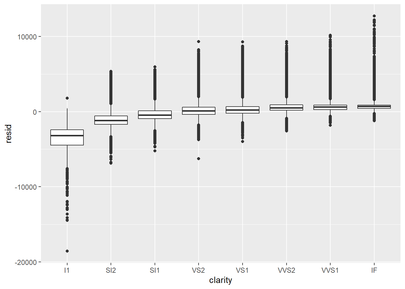
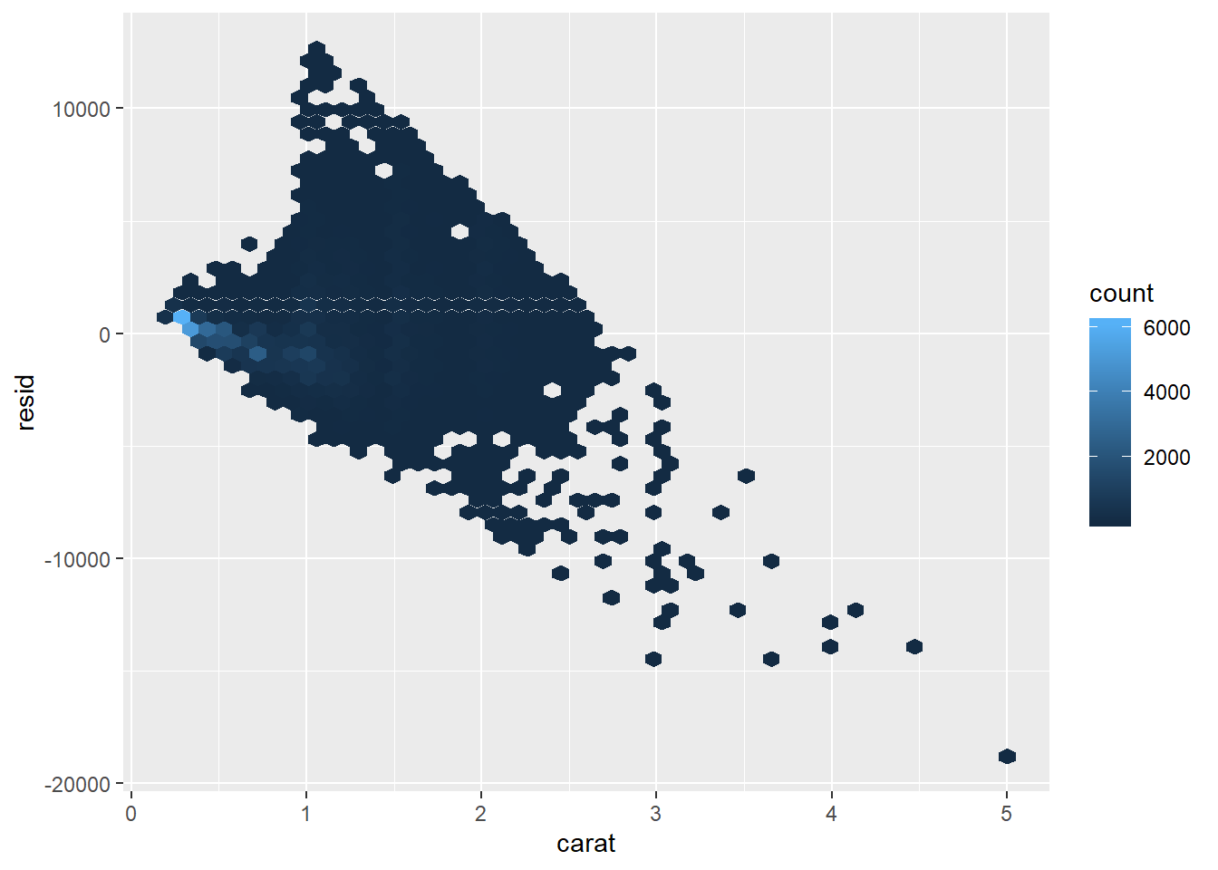
Now let us examine the residuals.

diamonds$resid <- residuals(mod_diamond)
ggplot(diamonds, aes(cut, resid)) + geom_boxplot()

ggplot(diamonds, aes(color, resid)) + geom_boxplot()

ggplot(diamonds, aes(clarity, resid)) + geom_boxplot()

5.4 Exercises

For the following exercises, you are expected to send me both your R script and a pdf document with your plots and interpretations.

Let us examine the residuals of our OLS model.

ggplot(diamonds, aes(carat, resid)) + 
  geom_hex(bins = 50)

Our model does not apprear to fit the data well. What are the possible reasons?
Can you improve our estimation by addressing these potential issues? Write up your R code and present your results.
Interpret what the three boxplots of diamond quality vs. residuals tell us.

Now, building on the reasons that you have identified, let us run a multiple regression using all four predictors.

Plot the relationship between diamond size and the residuals.
Plot the relationships between diamond quality and predicted prices.
Intrepret what you see from the plots.

5.5 Acknowledgement

This section is drawn from R for Data Science by Hadley Wickham and Computing for the Social Science by Benjamin Soltoff.