Chapter 6 Fixed or random effects
This section was originally prepared for the Adanced Methods of Political Analysis (Poli 706) in Spring 2019, which I served as a TA for Tobias Heinrich. The goal of this part is to address one common question we encounter in our research: when to use fixed or random effects?
6.1 Prerequisite
Load the following packages for this section.
library(modelr)
library(tidyverse)
library(foreign)
library(plm)
6.2 Introduction
Let us write down the following model (from Wooldridge p.435).
\(y_{it}=\beta_{1}x_{it} + a_{i} + u_{it}\)
Essentially, we have some “fixed” errors (\(a_{i}\)) over time. When we add the additional assumption that \(a_{i}\) is uncorrelated with any explanatory variable, we have the random effects model.
Let us get started by using the following data to run a simple OLS.
Panel <- read.dta("http://dss.princeton.edu/training/Panel101.dta")
ols <-lm(y ~ x1, data=Panel)
Now plot the fitted line.
grid <- data.frame(Intercept=1, x1=seq_range(Panel$x1, 10))
grid$pred <- predict(ols,grid)
ggplot(Panel, aes(x1)) +
  geom_point(aes(y = y)) +
  geom_line(aes(y = pred), data = grid, colour = "red", size = 1)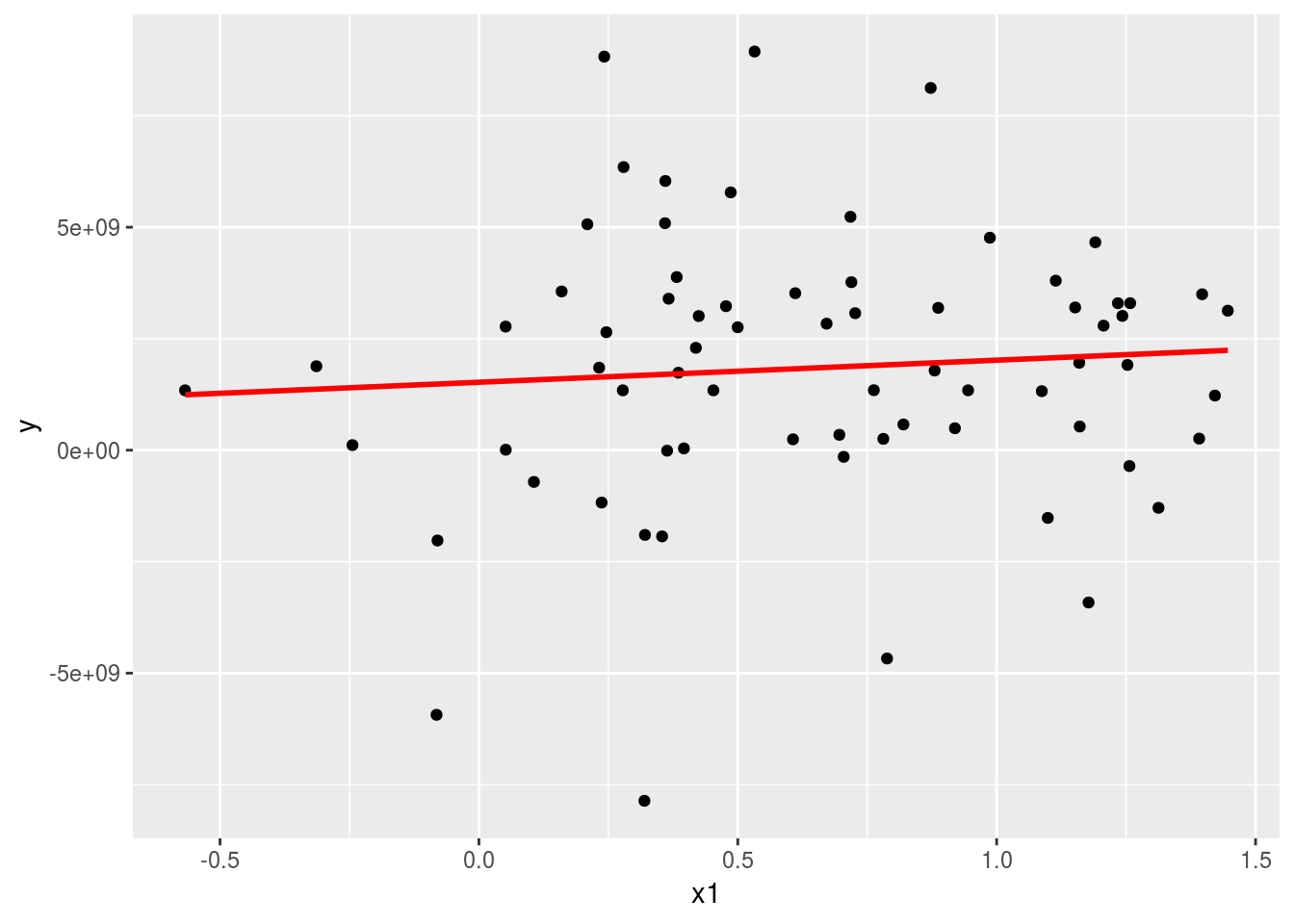
6.3 Fixed effects
There are two common ways to fit fixed effects. The first one is to addd dummy variables for the group indicator.
fixed_dum <-lm(y ~ x1 + factor(country) - 1, data=Panel)
summary(fixed_dum)
##
## Call:
## lm(formula = y ~ x1 + factor(country) - 1, data = Panel)
##
## Residuals:
## Min 1Q Median 3Q Max
## -8.634e+09 -9.697e+08 5.405e+08 1.386e+09 5.612e+09
##
## Coefficients:
## Estimate Std. Error t value Pr(>|t|)
## x1 2.476e+09 1.107e+09 2.237 0.02889 *
## factor(country)A 8.805e+08 9.618e+08 0.916 0.36347
## factor(country)B -1.058e+09 1.051e+09 -1.006 0.31811
## factor(country)C -1.723e+09 1.632e+09 -1.056 0.29508
## factor(country)D 3.163e+09 9.095e+08 3.478 0.00093 ***
## factor(country)E -6.026e+08 1.064e+09 -0.566 0.57329
## factor(country)F 2.011e+09 1.123e+09 1.791 0.07821 .
## factor(country)G -9.847e+08 1.493e+09 -0.660 0.51190
## ---
## Signif. codes: 0 '***' 0.001 '**' 0.01 '*' 0.05 '.' 0.1 ' ' 1
##
## Residual standard error: 2.796e+09 on 62 degrees of freedom
## Multiple R-squared: 0.4402, Adjusted R-squared: 0.368
## F-statistic: 6.095 on 8 and 62 DF, p-value: 8.892e-06grid_fixdum <- expand(data.frame(Intercept=1, x1=seq_range(Panel$x1, 14), country=unique(Panel$country)),
x1, country)
grid_fixdum$pred <- predict(fixed_dum,grid_fixdum)
ggplot(Panel, aes(x1)) +
geom_point(aes(y = y, colour=country)) +
geom_smooth(aes(y = y), method='lm', se=FALSE, colour="black")+
geom_line(data=grid_fixdum, aes(x=x1, y=pred, colour=country))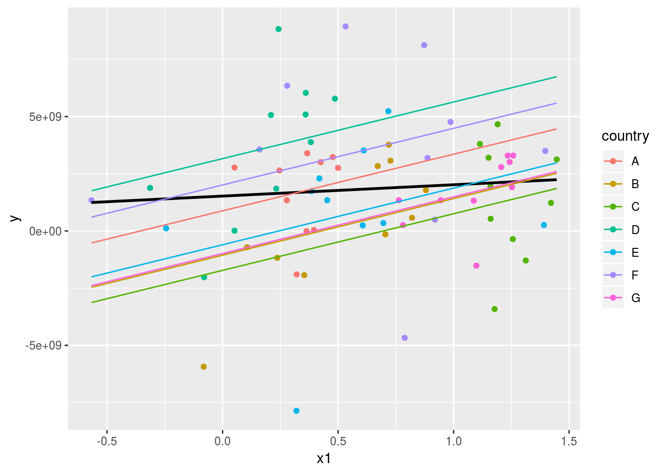
The second way is to incorporate fixed effects directly. In R, it is typically referred to as “within” model.
fixed <- plm(y ~ x1, data=Panel, index=c("country", "year"), model="within")
summary(fixed)
## Oneway (individual) effect Within Model
##
## Call:
## plm(formula = y ~ x1, data = Panel, model = "within", index = c("country",
## "year"))
##
## Balanced Panel: n = 7, T = 10, N = 70
##
## Residuals:
## Min. 1st Qu. Median Mean 3rd Qu. Max.
## -8.63e+09 -9.70e+08 5.40e+08 0.00e+00 1.39e+09 5.61e+09
##
## Coefficients:
## Estimate Std. Error t-value Pr(>|t|)
## x1 2475617827 1106675594 2.237 0.02889 *
## ---
## Signif. codes: 0 '***' 0.001 '**' 0.01 '*' 0.05 '.' 0.1 ' ' 1
##
## Total Sum of Squares: 5.2364e+20
## Residual Sum of Squares: 4.8454e+20
## R-Squared: 0.074684
## Adj. R-Squared: -0.029788
## F-statistic: 5.00411 on 1 and 62 DF, p-value: 0.028892We can then extract the fixed effects.
fixef(fixed) ## A B C D E F
## 880542404 -1057858363 -1722810755 3162826897 -602622000 2010731793
## G
## -984717493We can also test whether the fixed effects model is better than OLS.
pFtest(fixed, ols) ##
## F test for individual effects
##
## data: y ~ x1
## F = 2.9655, df1 = 6, df2 = 62, p-value = 0.01307
## alternative hypothesis: significant effects6.4 Random effects
random <- plm(y ~ x1, data=Panel, index=c("country", "year"), model="random")
summary(random)
## Oneway (individual) effect Random Effect Model
## (Swamy-Arora's transformation)
##
## Call:
## plm(formula = y ~ x1, data = Panel, model = "random", index = c("country",
## "year"))
##
## Balanced Panel: n = 7, T = 10, N = 70
##
## Effects:
## var std.dev share
## idiosyncratic 7.815e+18 2.796e+09 0.873
## individual 1.133e+18 1.065e+09 0.127
## theta: 0.3611
##
## Residuals:
## Min. 1st Qu. Median Mean 3rd Qu. Max.
## -8.94e+09 -1.51e+09 2.82e+08 0.00e+00 1.56e+09 6.63e+09
##
## Coefficients:
## Estimate Std. Error z-value Pr(>|z|)
## (Intercept) 1037014284 790626206 1.3116 0.1896
## x1 1247001782 902145601 1.3823 0.1669
##
## Total Sum of Squares: 5.6595e+20
## Residual Sum of Squares: 5.5048e+20
## R-Squared: 0.02733
## Adj. R-Squared: 0.013026
## Chisq: 1.91065 on 1 DF, p-value: 0.166896.4.1 Fixed or random
You can run a Hausman test (which tests whether the unique errors are correlated with the regressors, the null is they are not). If the p-value is significant, then you choose fixed effects (since the unique errors are correlated with the regressors).
phtest(fixed, random)##
## Hausman Test
##
## data: y ~ x1
## chisq = 3.674, df = 1, p-value = 0.05527
## alternative hypothesis: one model is inconsistent6.5 More tests
You can also add time fixed effects.
fixed_time_dum <- plm(y ~ x1 + factor(year), data=Panel, index=c("country", "year"), model="within")
summary(fixed_time_dum)
## Oneway (individual) effect Within Model
##
## Call:
## plm(formula = y ~ x1 + factor(year), data = Panel, model = "within",
## index = c("country", "year"))
##
## Balanced Panel: n = 7, T = 10, N = 70
##
## Residuals:
## Min. 1st Qu. Median Mean 3rd Qu. Max.
## -7.92e+09 -1.05e+09 -1.40e+08 0.00e+00 1.63e+09 5.49e+09
##
## Coefficients:
## Estimate Std. Error t-value Pr(>|t|)
## x1 1389050354 1319849567 1.0524 0.29738
## factor(year)1991 296381558 1503368528 0.1971 0.84447
## factor(year)1992 145369666 1547226548 0.0940 0.92550
## factor(year)1993 2874386795 1503862554 1.9113 0.06138 .
## factor(year)1994 2848156288 1661498927 1.7142 0.09233 .
## factor(year)1995 973941306 1567245748 0.6214 0.53698
## factor(year)1996 1672812557 1631539254 1.0253 0.30988
## factor(year)1997 2991770063 1627062032 1.8388 0.07156 .
## factor(year)1998 367463593 1587924445 0.2314 0.81789
## factor(year)1999 1258751933 1512397632 0.8323 0.40898
## ---
## Signif. codes: 0 '***' 0.001 '**' 0.01 '*' 0.05 '.' 0.1 ' ' 1
##
## Total Sum of Squares: 5.2364e+20
## Residual Sum of Squares: 4.0201e+20
## R-Squared: 0.23229
## Adj. R-Squared: 0.00052851
## F-statistic: 1.60365 on 10 and 53 DF, p-value: 0.13113Or simply,
fixed_time <- plm(y ~ x1, data=Panel, index=c("country", "year"), model="within", effect="twoway")
summary(fixed_time)
## Twoways effects Within Model
##
## Call:
## plm(formula = y ~ x1, data = Panel, effect = "twoway", model = "within",
## index = c("country", "year"))
##
## Balanced Panel: n = 7, T = 10, N = 70
##
## Residuals:
## Min. 1st Qu. Median Mean 3rd Qu. Max.
## -7.92e+09 -1.05e+09 -1.40e+08 0.00e+00 1.63e+09 5.49e+09
##
## Coefficients:
## Estimate Std. Error t-value Pr(>|t|)
## x1 1389050354 1319849567 1.0524 0.2974
##
## Total Sum of Squares: 4.1041e+20
## Residual Sum of Squares: 4.0201e+20
## R-Squared: 0.020471
## Adj. R-Squared: -0.27524
## F-statistic: 1.10761 on 1 and 53 DF, p-value: 0.297386.5.1 Test whether adding time-fixed effects is necessary
pFtest(fixed_time, fixed)or (a note for myself, plmtest cannot be deployed into the website as it causes errors, which is odd since other people seem to be able to deploy)
plmtest(fixed, effect="time", type="bp")6.5.2 Test between OLS and random effects
pool <- plm(y ~ x1, data=Panel, index=c("country", "year"), model="pooling")
plmtest(pool, effect="individual", type="bp")
6.5.3 Test cross-sectional dependence (contemporaneous correlation)
pcdtest(fixed, test = c("lm"))
pcdtest(fixed, test = c("cd"))
6.5.4 Test for serial correlation
pbgtest(fixed)6.5.5 Test for stationarity
Panel_set <- pdata.frame(Panel, index = c("country", "year"))
library(tseries)
adf.test(Panel_set$y, k=2)
6.5.6 Test for heteroskedasticity
library(lmtest)
bptest(y ~ x1 + factor(country), data = Panel, studentize=F)
To address heteroskedasticity, you can use robust standard errors.
coeftest(fixed)
coeftest(fixed, vcovHC)
There are different types of estimators and options to choose from.
coeftest(fixed, vcovHC(fixed, method = "arellano"))
t(sapply(c("HC0", "HC1", "HC2", "HC3", "HC4"), function(x) sqrt(diag(vcovHC(fixed, method = "arellano", type = x)))))
Here are some suggestions from Oscar Torres-Reyna’s tutorial.
The –vcovHC– function estimates three heteroskedasticity-consistent covariance estimators:
- “white1” - for general heteroskedasticity but no serial correlation. Recommended for random effects.
- “white2” - is “white1” restricted to a common variance within groups. Recommended for random effects.
- “arellano” - both heteroskedasticity and serial correlation. Recommended for fixed effects.
The following options apply:
- HC0 - heteroskedasticity consistent. The default.
- HC1,HC2, HC3 – Recommended for small samples. HC3 gives less weight to influential observations.
- HC4 - small samples with influential observations
- HAC - heteroskedasticity and autocorrelation consistent (type ?vcovHAC for more details)
For more details, see here at page 4.
6.6 Additional reading
Brandon Bartels offers some suggestions for analyzing multilevel data here. See here for Andrew Gelman’s take.
If you find the use of fixed vs. random effects confusing or unsatisfying, I would highly recommend Gelman and Hill’s book Data Analysis Using Regression and Multilevel/Hierarchical Models, where they urge us to avoid using the term “fixed” and “random” entirely. In particular, you should read at least chapter 11 and 12.
6.7 Acknowledgement
This section is drawn from Princeton’s Getting Started in Fixed/Random Effects Models using R by Oscar Torres-Reyna.