4 When $β$ s vary among groups: multilevel linear model

Multilevel linear model is also known as random coefficients model (RCM), linear mixed model (LMM), and hierarchical linear model (HLM).

4.1 Multilevel data and heterogeneity (non-dependence)

Following are two real data examples.

Repeated measure design.

The sleepstudy data set in the lme4 packages, containing the average reaction time per day (in milliseconds) for 18 subjects in a sleep deprivation study over 10 days (day 0-day 9):

ABCDEFGHIJ0123456789

	Reaction <dbl>	Days <dbl>	Subject <fct>
1	249.5600	0	308
2	258.7047	1	308
3	250.8006	2	308
4	321.4398	3	308
5	356.8519	4	308
6	414.6901	5	308

Overall, the average reaction time increase in days. However, we observe great heterogeneity. If we fitted multiple linear regression to the data of each individual, the resulting regression lines vary markedly in that different subject has different intercepts and slopes. More specifically, we observe wider variation in slopes than in intercepts.

Hierarchical design: nested in cluster.

Data are from Barcikowski (1981), High School & Beyond Survey, a data set from a nationally representative sample of U.S. public and Catholic high schools. 7185 students nested within 160 schools.

DV: mathach, math achievement,
IV:
- ses, social economic status,
- sector, public school vs Catholic school.
- ID, school.

ABCDEFGHIJ0123456789

	ID <int>	mathach <dbl>	ses <dbl>	sector <chr>
1	1224	5.876	-1.528	Public
2	1224	19.708	-0.588	Public
3	1224	20.349	-0.528	Public
4	1224	8.781	-0.668	Public
5	1224	17.898	-0.158	Public
6	1224	4.583	0.022	Public

It is clearly shown that different schools have different slopes and intercepts, implying school-level heterogeneity that is completely masked by multiple linear regression.

Heterogeneity sometimes refers to non-dependence. For example, students in the same school share similar environment (same math textbook, same math teacher, same study body, etc.), thus students tend to have math achievement similar to their peers from the same school than those from other school. Put another way, data are independent within school but not independent across school.

So why not fitting multiple linear regression to each group? If so, we wind up with smaller sample size and consequently lower statistical power for each regression models. Multilevel linear model uses all $n$ observations and takes heterogeneity into account by modeling regression coefficients (intercept and slopes) as random variables. Not surprisingly, multilevel linear model enjoys better model fit due to incorporating underlying heterogeneity of data.

4.2 The basic multilevel linear model

Random intercept and random slopes

$\begin{aligned} Level 1: y_{i j} & = β_{0 j} + β_{1 j} x_{1 i j} + \dots + β_{p j} x_{p i j} + ϵ_{i j} \\ Level 2: β_{0 j} & = γ_{00} + u_{0 j} \\ Level 2: β_{1 j} & = γ_{10} + u_{1 j} \\ \dots \\ Level 2: β_{p j} & = γ_{p 0} + u_{p j} \\ Mixed: y_{i j} & = γ_{00} + (γ_{10} x_{1 i j} + \dots + γ_{p 0} x_{p i j}) + \\ (u_{1 j} x_{1 i j} + \dots + u_{p j} x_{p i j}) + u_{0 j} + ϵ_{i j}, \end{aligned}$ where $blue$ terms are fixed effects, $red$ terms are random effects, $j = 1, \dots, m$ represents grouping variable (i.e., subject in sleepstudy data, and sector in Barcikowsk’s data), $i = 1, \dots, n_{j}$ represents observation (i.e., subject) within $j$ th group, total sample size $n = n_{1} + \dots + n_{m}$ , $x_{1}$ , $\dots$ , $x_{p}$ are $p$ independent variables, $y$ is dependent variable, $ϵ_{i j} \sim i i d N (0, σ_{ϵ}^{2})$ , $\begin{array}{r} (\begin{array}{c} u_{0 j} \\ u_{1 j} \\ ⋮ \\ u_{p j} \end{array}) \sim M V N (0, Σ_{u}), Σ_{u} = [\begin{array}{c} σ_{u_{0 j}}^{2} \\ σ_{u_{1 j}, u_{0 j}} & σ_{u_{1 j}}^{2} \\ ⋮ & ⋮ & ⋱ \\ σ_{u_{p j}, u_{0 j}} & σ_{u_{p j}, u_{1 j}} & \dots & σ_{u_{p j}}^{2} \end{array}] . \end{array}$ In this model,

Random intercept only

$\begin{aligned} Level 1: y_{i j} & = β_{0 j} + β_{1} x_{1 i j} + \dots + β_{p} x_{p i j} + ϵ_{i j} \\ Level 2: β_{0 j} & = γ_{00} + u_{0 j} \\ Mixed: y_{i j} & = γ_{00} + β_{1} x_{1 i j} + \dots + β_{p} x_{p i j} + u_{0 j} + ϵ_{i j}, \end{aligned}$ where $u_{0 j} \sim N (0, σ_{u_{0 j}}^{2})$ .

Random slopes only

$\begin{aligned} Level 1: y_{i j} & = β_{0} + β_{1 j} x_{1 i j} + \dots + β_{p j} x_{p i j} + ϵ_{i j} \\ Level 2: β_{1 j} & = γ_{10} + u_{1 j} \\ \dots \\ Level 2: β_{p j} & = γ_{p 0} + u_{p j} \\ Mixed: y_{i j} & = β_{0} + (γ_{10} x_{1 i j} + \dots + γ_{p 0} x_{p i j}) + (u_{1 j} x_{1 i j} + \dots + u_{p j} x_{p i j}) + ϵ_{i j}, \end{aligned}$ where $\begin{array}{r} (\begin{array}{c} u_{1 j} \\ ⋮ \\ u_{p j} \end{array}) \sim M V N (0, Σ_{u}), Σ_{u} = [\begin{array}{c} σ_{u_{1 j}}^{2} \\ ⋮ & ⋱ \\ σ_{u_{p j}, u_{1 j}} & \dots & σ_{u_{p j}}^{2} \end{array}] . \end{array}$

Suppose we only have 1 $x$ and 1 $y$ :

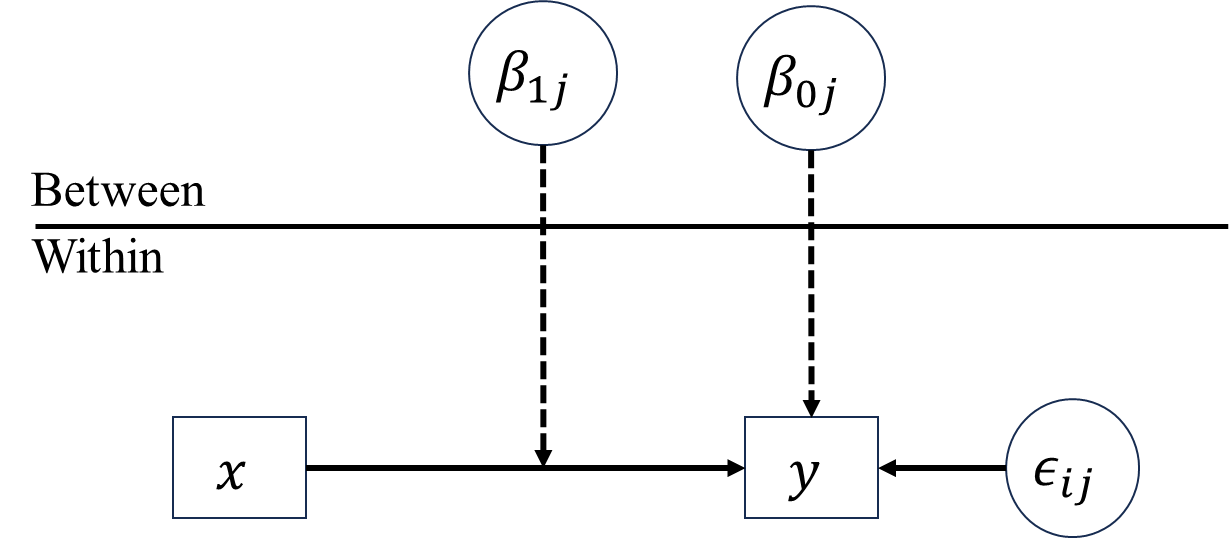
Random intercept and random slope

$\begin{aligned} Level 1: y_{i j} & = β_{0 j} + β_{1 j} x_{i j} + ϵ_{i j} \\ Level 2: β_{0 j} & = γ_{00} + u_{0 j} \\ Level 2: β_{1 j} & = γ_{10} + u_{1 j} \\ Mixed: y_{i j} & = γ_{00} + γ_{10} x_{i j} + u_{1 j} x_{i j} + u_{0 j} + ϵ_{i j}, \end{aligned}$ where $\begin{array}{r} (\begin{array}{c} u_{0 j} \\ u_{1 j} \end{array}) \sim [\begin{array}{c} σ_{u_{0 j}}^{2} \\ σ_{u_{1 j}, u_{0 j}} & σ_{u_{1 j}}^{2} \end{array}] . \end{array}$

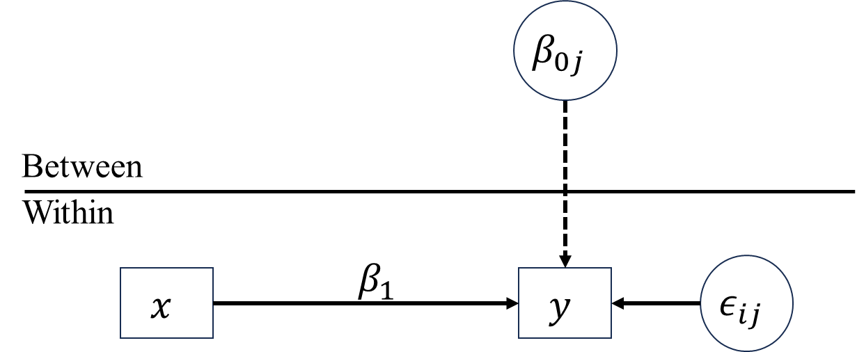
Random intercept only

$\begin{aligned} Level 1: y_{i j} & = β_{0 j} + β_{1} x_{i j} + ϵ_{i j} \\ Level 2: β_{0 j} & = γ_{00} + u_{0 j} \\ Mixed: y_{i j} & = γ_{00} + β_{1} x_{i j} + u_{0 j} + ϵ_{i j}, \end{aligned}$ where $u_{0 j} \sim N (0, σ_{u_{0 j}}^{2})$ .

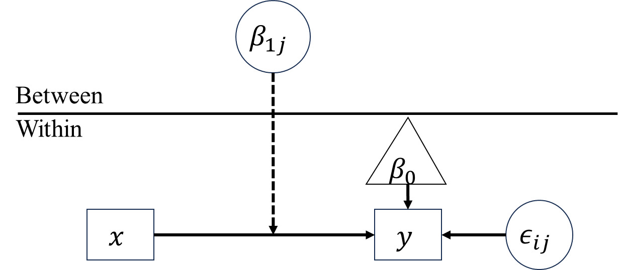
Random slope only

$\begin{aligned} Level 1: y_{i j} & = β_{0} + β_{1 j} x_{i j} + ϵ_{i j} \\ Level 2: β_{1 j} & = γ_{10} + u_{1 j} \\ Mixed: y_{i j} & = β_{0} + γ_{10} x_{i j} + u_{1 j} x_{i j} + ϵ_{i j}, \end{aligned}$ where $u_{1 j} \sim N (0, σ_{u_{1 j}}^{2})$ .

Quiz: why allowing the lower-triangular parts of $Σ_{u}$ to be freely estimated?

4.3 Syntax style

Mplus: multilevel model
lme4: linear mixed model

4.4 Variance decomposition and intra-class correlation (ICC)

4.4.1 Variance decomposition

Random intercept and random slopes

$\begin{aligned} Mixed: y_{i j} & = γ_{00} + (γ_{10} x_{1 i j} + \dots + γ_{p 0} x_{p i j}) + \\ (u_{1 j} x_{1 i j} + \dots + u_{p j} x_{p i j}) + u_{0 j} + ϵ_{i j} \\ Var (y_{i j}) & = Var (u_{1 j} x_{1 i j} + \dots + u_{p j} x_{p i j} + u_{0 j} + ϵ_{i j}) \\ = x_{1 i j}^{2} σ_{u_{1 j}}^{2} + \dots + x_{p i j}^{2} σ_{u_{p j}}^{2} + σ_{u_{0 j}}^{2} + \\ 2 \sum_{k^{'} = k + 1}^{p} \sum_{k = 1}^{p - 1} x_{k i j} x_{k^{'} i j} σ_{u_{k j}, u_{k^{'} j}} + 2 \sum_{k}^{p} x_{k i j} σ_{u_{k j}, u_{0 j}} + \\ σ_{ϵ_{i j}}^{2} \\ = σ_{B}^{2} + σ_{W}^{2} . \end{aligned}$ where $σ_{B}^{2}$ is the between-group variance and $σ_{W}^{2}$ is the within-group variance, since $e_{i j}$ is random error, it is assumed to be independent to all other random terms, therefore, $σ_{u_{0 j}, e_{i j}} = σ_{u_{k j}, e_{i j}} = 0$ .

Random intercept only

$\begin{aligned} Mixed: y_{i j} & = γ_{00} + β_{1} x_{1 i j} + \dots + β_{p} x_{p i j} + u_{0 j} + ϵ_{i j} \\ Var (y_{i j}) & = Var (u_{0 j} + ϵ_{i j}) \\ = σ_{u_{0 j}}^{2} + σ_{ϵ_{i j}}^{2} . \end{aligned}$

Random slopes only

$\begin{aligned} Mixed: y_{i j} & = β_{0} + (γ_{10} x_{1 i j} + \dots + γ_{p 0} x_{p i j}) + (u_{1 j} x_{1 i j} + \dots + u_{p j} x_{p i j}) + ϵ_{i j} \\ Var (y_{i j}) & = Var (u_{1 j} x_{1 i j} + \dots + u_{p j} x_{p i j} + ϵ_{i j}) \\ = x_{1 i j}^{2} σ_{u_{1 j}}^{2} + \dots + x_{p i j}^{2} σ_{u_{p j}}^{2} + 2 \sum_{k^{'} = k + 1}^{p} \sum_{k = 1}^{p - 1} x_{k i j} x_{k^{'} i j} σ_{u_{k j}, u_{k^{'} j}} + σ_{ϵ_{i j}}^{2} . \end{aligned}$ Suppose we only have 1 $x$ and 1 $y$ :

Random intercept and random slope

$\begin{aligned} Mixed: y_{i j} & = γ_{00} + γ_{10} x_{i j} + u_{1 j} x_{i j} + u_{0 j} + ϵ_{i j} \\ Var (y_{i j}) & = Var (u_{1 j} x_{i j} + u_{0 j} + ϵ_{i j}) \\ = x_{i j}^{2} σ_{u_{1 j}}^{2} + σ_{u_{0 j}}^{2} + 2 x_{i j} σ_{u_{1 j}, u_{0 j}} + σ_{ϵ_{i j}}^{2} . \end{aligned}$

Random intercept only

$\begin{aligned} Mixed: y_{i j} & = γ_{00} + β_{1} x_{i j} + u_{0 j} + ϵ_{i j} \\ Var (y_{i j}) & = Var (u_{0 j} + ϵ_{i j}) \\ = σ_{u_{0 j}}^{2} + σ_{ϵ_{i j}}^{2} . \end{aligned}$

Random random slope only

$\begin{aligned} Mixed: y_{i j} & = β_{0} + γ_{10} x_{i j} + u_{1 j} x_{i j} + ϵ_{i j} \\ Var (y_{i j}) & = Var (u_{1 j} x_{i j} + ϵ_{i j}) \\ = x_{i j}^{2} σ_{u_{1 j}}^{2} + σ_{ϵ_{i j}}^{2} . \end{aligned}$

4.4.2 Intra-class correlation (ICC)

An convenient summary of the “importance” of grouping variables is the proportion of the total variance accounted for, denoted as variance partition coefficient (VPC) $\begin{aligned} V P C & = \frac{σ_{B}^{2}}{σ_{B}^{2} + σ_{W}^{2}} . \end{aligned}$ For multilevel linear model with random slopes, VPC becomes a function of $x$ s. For example, by fitting a multilevel model with both random intercept and slope to the sleepstudy data while fixing the corvariance between the error term , we have $\begin{aligned} Level 1: R e a c t i o n_{i j} & = β_{0 j} + β_{1 j} D a y s_{i j} + ϵ_{i j} \\ Level 2: β_{0 j} & = γ_{00} + u_{0 j} \\ Level 2: β_{1 j} & = γ_{10} + u_{1 j}, \end{aligned}$ $σ_{u_{0 j}, u_{1 j}} = 0$ . Base on the estimated parameters, we can draw the following scatter plot,

#> Linear mixed model fit by REML. t-tests use Satterthwaite's method [
#> lmerModLmerTest]
#> Formula: Reaction ~ Days + (Days || Subject)
#>    Data: sleepstudy
#> 
#> REML criterion at convergence: 1743.7
#> 
#> Scaled residuals: 
#>     Min      1Q  Median      3Q     Max 
#> -3.9626 -0.4625  0.0204  0.4653  5.1860 
#> 
#> Random effects:
#>  Groups    Name        Variance Std.Dev.
#>  Subject   (Intercept) 627.57   25.051  
#>  Subject.1 Days         35.86    5.988  
#>  Residual              653.58   25.565  
#> Number of obs: 180, groups:  Subject, 18
#> 
#> Fixed effects:
#>             Estimate Std. Error      df t value Pr(>|t|)    
#> (Intercept)  251.405      6.885  18.156  36.513  < 2e-16 ***
#> Days          10.467      1.560  18.156   6.712 2.59e-06 ***
#> ---
#> Signif. codes:  0 '***' 0.001 '**' 0.01 '*' 0.05 '.' 0.1 ' ' 1
#> 
#> Correlation of Fixed Effects:
#>      (Intr)
#> Days -0.184

#>  Groups    Name        Std.Dev.
#>  Subject   (Intercept) 25.0513 
#>  Subject.1 Days         5.9882 
#>  Residual              25.5653

Intra-class correlation (ICC) is defined as $\begin{aligned} I C C & = \frac{σ_{u_{0 j}}^{2}}{σ_{u_{0 j}}^{2} + σ_{W}^{2}} . \end{aligned}$ For a random intercept only model, ICC = VPC, otherwise ICC is a biased estimator of VPC, thus the common practice is reporting variance components.

Based on ICC we can calculate the reliability of $j$ th group (Heck & Thomas, 2020, equation 3.5) $\begin{aligned} λ_{j} & = \frac{σ_{u_{0 j}}^{2}}{σ_{u_{0 j}}^{2} + σ_{W}^{2} / n_{j}} . \end{aligned}$

Reference:

4.5 Effects decomposition and centering

4.5.1 Within effect, between effect, contextual effect

Within effect describes the relationship between within-level background variables and within-level outcome variable. For example, how does student’s ses impact their math achievement within a given school?

Contextual effect describes the impact of the context on the relationship between between-level background variable (i.e. group mean ses) and within-level outcome variable (i.e. math achievement). In the Barcikowski’s data example, contextual effect explores whether two students from different schools with the same level of average ses have different levels of math achievement. Another classic example of contextual effect is the Big Fish-Little Pond effect (Marsh & Parker, 1984). This effect describes the situation in which high achieving students in a school that is low achieving on average, will feel better about their abilities than high achieving students in a school with higher average achievement.

Examples from Rönkkö’s video on within effect, between effect, contextual effect, and population average effect
Y	X	Group	Within effect	Contextual effect
Health	Vaccination (1 or 0)	Community	Positive: Within a specific community, getting vaccination decreases individual’s risk of contracting a disease	Positive: Community with higher vaccination rate (average vaccination) decreases its dweller’s risk of contracting a disease
Profits	Overfishing	Lake	Positive: Within a specific lake, if a professional fisherman exceeded his fishing quota, his profits will increase because of larger catch	Negative: Lake with higer level of overfishing (average overfishing), the profits of all fishmen will decrease because of smaller catches
Competitive advantage	Innovativeness	Industry	Positive: Within a industry, if a firm was innovative, it can develop valuable capabilities that lead to competitive advantage	Negative: Industry with higher level of innovativeness (average innovativeness) have more innovations, but innovativeness is less likely to lead to competitive advantage
Performance	Gender (1 or 0)	Team	Zero: Within a specific team, one’s gender has no effect one’s performance	Inverted U-shapde: Team with half mean and half women (medium level of average gender) works best

Between effect = within effect + contextual effect. Between effect describes the relationship between the group-level average background variables and the group-level average outcome variable. For example, how does a school’s average ses affect the average math achievement of the students in this school?

Multiple linear regression mixes the above effects together. In multilevel linear model, we can extract the three effects and further explain our findings. However, the way how these three effects are decomposed in a multilevel liear model is influenced by whether and how do we center our data.

4.5.2 Centering or not? that is the question.

4.5.2.1 Raw data

Let’s use Barcikowsk’s data as an example. With a multilevel linear model with both random slope and random intercept, fix the covariance between random intercept and random slope at 0, we have $\begin{aligned} Level 1: m a t h a c h_{i j} & = β_{0 j} + β_{1 j} s e s_{i j} + ϵ_{i j} \\ Level 2: β_{0 j} & = γ_{00} + u_{0 j} \\ Level 2: β_{1 j} & = γ_{10} + u_{1 j} \\ Mixed: m a t h a c h_{i j} & = γ_{00} + γ_{10} s e s_{i j} + u_{1 j} s e s_{i j} + u_{0 j} + ϵ_{i j}, \end{aligned}$

#> Linear mixed model fit by REML. t-tests use Satterthwaite's method [
#> lmerModLmerTest]
#> Formula: mathach ~ ses + (ses || ID)
#>    Data: Barcikowsk
#> 
#> REML criterion at convergence: 46640.7
#> 
#> Scaled residuals: 
#>      Min       1Q   Median       3Q      Max 
#> -3.12410 -0.73160  0.02253  0.75467  2.93201 
#> 
#> Random effects:
#>  Groups   Name        Variance Std.Dev.
#>  ID       (Intercept)  4.853   2.2029  
#>  ID.1     ses          0.424   0.6511  
#>  Residual             36.822   6.0681  
#> Number of obs: 7185, groups:  ID, 160
#> 
#> Fixed effects:
#>             Estimate Std. Error       df t value Pr(>|t|)    
#> (Intercept)  12.6527     0.1903 146.2881   66.50   <2e-16 ***
#> ses           2.3955     0.1184 158.8487   20.23   <2e-16 ***
#> ---
#> Signif. codes:  0 '***' 0.001 '**' 0.01 '*' 0.05 '.' 0.1 ' ' 1
#> 
#> Correlation of Fixed Effects:
#>     (Intr)
#> ses 0.000

In Barcikowsk’s data, $\hat{γ_{10}}$ is 2.3955, meaning that student’s $m a t h a c h$ increase 2.3955 with 1-unit increase in $s e s$ . However, this effect of $s e s$ on $m a t h a c h$ is actually a confounded version of the within- and between- effects. We shall leave the explanation to the end of Section 4.5.2.

To properly decompose them, we need to use $m e a n s e s_{j}$ as a between level predictor, $\begin{aligned} Level 1: m a t h a c h_{i j} & = β_{0 j} + β_{1 j} s e s_{i j} + ϵ_{i j} \\ Level 2: β_{0 j} & = γ_{00} + b_{01} m e a n s e s_{j} + u_{0 j} \\ Level 2: β_{1 j} & = γ_{10} + u_{1 j} \\ Mixed: m a t h a c h_{i j} & = γ_{00} + γ_{10} s e s_{i j} + b_{01} m e a n s e s_{j} + \\ u_{1 j} s e s_{i j} + u_{0 j} + ϵ_{i j} . \end{aligned}$

#> Linear mixed model fit by REML. t-tests use Satterthwaite's method [
#> lmerModLmerTest]
#> Formula: mathach ~ ses + mean_group_ses + (ses || ID)
#>    Data: Barcikowsk
#> 
#> REML criterion at convergence: 46562.4
#> 
#> Scaled residuals: 
#>      Min       1Q   Median       3Q      Max 
#> -3.15390 -0.72254  0.01774  0.75562  2.95378 
#> 
#> Random effects:
#>  Groups   Name        Variance Std.Dev.
#>  ID       (Intercept)  2.7129  1.6471  
#>  ID.1     ses          0.4835  0.6953  
#>  Residual             36.7793  6.0646  
#> Number of obs: 7185, groups:  ID, 160
#> 
#> Fixed effects:
#>                Estimate Std. Error       df t value Pr(>|t|)    
#> (Intercept)     12.6759     0.1510 153.1039  83.926   <2e-16 ***
#> ses              2.1923     0.1227 182.5178  17.867   <2e-16 ***
#> mean_group_ses   3.7762     0.3839 182.9834   9.836   <2e-16 ***
#> ---
#> Signif. codes:  0 '***' 0.001 '**' 0.01 '*' 0.05 '.' 0.1 ' ' 1
#> 
#> Correlation of Fixed Effects:
#>             (Intr) ses   
#> ses         -0.003       
#> mean_grp_ss  0.007 -0.258

$\hat{γ_{00}} = 12.6759$ is the predicted student’s $m a t h a c h$ when $s e s = 0$ and $m e a n s e s = 0$ , however, it makes no sense for $s e s$ and $m e a n s e s$ to be equal to 0, thus the intepretation of $\hat{γ_{00}}$ is lacking of practical meaning, for which centering can be a helping hand,
$γ_{10}$ is clearly the within effect. $\hat{γ_{10}} = 2.1923$ , meaning that student’s predicted $m a t h a c h$ increase 2.1923 with 1-unit increase in $s e s$ controlling $m e a n s e s$ , that is, if two students from the same school, $m e a n s e s$ remained constant, the difference of their predicted $m a t h a c h$ only depend on their $s e s$ s.
$b_{01}$ represents the contextual effect. $\hat{b_{01}} = 3.7762$ , meaning that student’s predicted $m a t h a c h$ increase 3.7762 with 1-unit increase in school’s $m e a n s e s$ controlling $s e s$ , that is, if two student having identical $s e s$ s, the difference of their predicted $m a t h a c h$ only depend on the $m e a n s e s$ of their school, thus $b_{01}$ represent the contextual effect.
between effect = 2.1923 + 3.7762 = 5.9685.

4.5.2.2 Centering in multiple linear regression

Centering change the scale of independent variable and facilitate the interpretation of intercept.

Note

Note that we only center background variables and leave the dependent variables in their orginal scale.

For example, suppose we fit a simple linear regression, with raw data we have $\begin{array}{r} y_{i} = β_{0} + β_{1} x_{i} + ϵ_{i}, \end{array}$ of which the intercept is interpretated as the prediction of $y$ when $x = 0$ . After centering $x$ we have $\begin{aligned} y_{i} & = β_{0} + β_{1} (x_{i} - \bar{x}) + ϵ_{i} \\ y_{i} & = β_{0} + β_{1} (x c_{i}) + ϵ_{i}, \end{aligned}$ of which the intercept is interpretated as the prediction of $y$ when $x c_{i} = 0$ , i.e. $x_{i} = \bar{x}$ .

In multilevel linear model, there are basically two types of centering strategies for the within level background variables, grand-mean centering (GMC) and group-mean centering, aka cluster-mean centering (CMC). CMC is used throughout this chapter to avoid identical initials.

4.5.2.3 Grand-mean centering (GMC)

Let’s fit a multilevel linear model with both random slope and random intercept to Barcikowsk’s data, and fix the covariance between random intercept and random slope at 0. $s e s$ now is grand-mean centered. $\begin{aligned} Level 1: m a t h a c h_{i j} & = β_{0 j} + β_{1 j} s e s G M C_{i j} + ϵ_{i j} \\ Level 2: β_{0 j} & = γ_{00} + u_{0 j} \\ Level 2: β_{1 j} & = γ_{10} + u_{1 j} \\ Mixed: y_{i j} & = γ_{00} + γ_{10} s e s G M C_{i j} + u_{1 j} s e s G M C_{i j} + u_{0 j} + ϵ_{i j}, \end{aligned}$ $γ_{00}$ represents the predicted $m a t h a c h$ when $s e s$ equal to the grand mean, $γ_{10}$ represents the change in $m a t h a c h$ given 1-unit change in $s e s G M C$ .

#> Linear mixed model fit by REML. t-tests use Satterthwaite's method [
#> lmerModLmerTest]
#> Formula: mathach ~ I(ses - mean_grand_ses) + (ses || ID)
#>    Data: Barcikowsk
#> 
#> REML criterion at convergence: 46640.7
#> 
#> Scaled residuals: 
#>      Min       1Q   Median       3Q      Max 
#> -3.12410 -0.73160  0.02253  0.75467  2.93201 
#> 
#> Random effects:
#>  Groups   Name        Variance Std.Dev.
#>  ID       (Intercept)  4.853   2.2029  
#>  ID.1     ses          0.424   0.6511  
#>  Residual             36.822   6.0681  
#> Number of obs: 7185, groups:  ID, 160
#> 
#> Fixed effects:
#>                         Estimate Std. Error       df t value Pr(>|t|)    
#> (Intercept)              12.6531     0.1903 146.2881   66.50   <2e-16 ***
#> I(ses - mean_grand_ses)   2.3955     0.1184 158.8487   20.23   <2e-16 ***
#> ---
#> Signif. codes:  0 '***' 0.001 '**' 0.01 '*' 0.05 '.' 0.1 ' ' 1
#> 
#> Correlation of Fixed Effects:
#>             (Intr)
#> I(-mn_grn_) 0.000

Similarly, without $m e a n s e s$ in the between level, we are unable to decompose within- and between- effect.

Note

Note that, it is usually recommended to grand-mean center the group mean variable before adding it to between level for better interpretation.

$\begin{aligned} Level 1: m a t h a c h_{i j} & = β_{0 j} + β_{1 j} s e s G M C_{i j} + ϵ_{i j} \\ Level 2: β_{0 j} & = γ_{00} + b_{01} m e a n s e s_{j} + u_{0 j} \\ Level 2: β_{1 j} & = γ_{10} + u_{1 j} \\ Mixed: y_{i j} & = γ_{00} + γ_{10} s e s G M C_{i j} + b_{01} m e a n s e s G M C_{j} + \\ u_{1 j} s e s G M C_{i j} + u_{0 j} + ϵ_{i j} . \end{aligned}$

#> Linear mixed model fit by REML. t-tests use Satterthwaite's method [
#> lmerModLmerTest]
#> Formula: mathach ~ I(ses - mean_grand_ses) + mean_group_ses_cen + (ses ||  
#>     ID)
#>    Data: Barcikowsk
#> 
#> REML criterion at convergence: 46562.4
#> 
#> Scaled residuals: 
#>      Min       1Q   Median       3Q      Max 
#> -3.15390 -0.72254  0.01774  0.75562  2.95378 
#> 
#> Random effects:
#>  Groups   Name        Variance Std.Dev.
#>  ID       (Intercept)  2.7129  1.6471  
#>  ID.1     ses          0.4835  0.6953  
#>  Residual             36.7793  6.0646  
#> Number of obs: 7185, groups:  ID, 160
#> 
#> Fixed effects:
#>                         Estimate Std. Error       df t value Pr(>|t|)    
#> (Intercept)              12.6767     0.1510 153.1025  83.931   <2e-16 ***
#> I(ses - mean_grand_ses)   2.1923     0.1227 182.5178  17.867   <2e-16 ***
#> mean_group_ses_cen        3.7762     0.3839 182.9834   9.836   <2e-16 ***
#> ---
#> Signif. codes:  0 '***' 0.001 '**' 0.01 '*' 0.05 '.' 0.1 ' ' 1
#> 
#> Correlation of Fixed Effects:
#>             (Intr) I(-m__
#> I(-mn_grn_) -0.003       
#> mn_grp_ss_c  0.007 -0.258

$\hat{γ_{00}} = 12.6767$ is the prediction of $m a t h a c h$ when $s e s G M C = 0$ ( $s e s_{i j}$ is equal to the grand mean) and $m e a n s e s G M C = 0$ ( $m e a n s e s$ is equal to the average $m e a n s e s$ of all schools),
Within effect: $\hat{γ_{10}} = 2.1923$ , meaning that student’s predicted $m a t h a c h$ increase 2.1923 with 1-unit increase in $s e s G M C$ controlling $m e a n s e s G M C$ , that is, if two students from the same school, $m e a n s e s G M C$ remained constant, the difference of their predicted $m a t h a c h$ only depend on their $s e s G M C$ s.
Contextual effect: $\hat{b_{01}} = 3.7762$ , meaning that student’s predicted $m a t h a c h$ increase 3.7762 with 1-unit increase in school’s $m e a n s e s G M C$ controlling $s e s G M C$ , that is, if two student having identical $s e s G M C$ s, the difference of their predicted $m a t h a c h$ only depend on the $m e a n s e s G M C$ of their school, thus $b_{01}$ represent the contextual effect.
Between effect = 2.1923 + 3.7762 = 5.9685.

4.5.2.4 Cluster-mean centering (CMC)

Centering $s e s$ with cluster-mean we have $\begin{aligned} Level 1: m a t h a c h_{i j} & = β_{0 j} + β_{1 j} s e s C M C_{i j} + ϵ_{i j} \\ Level 2: β_{0 j} & = γ_{00} + u_{0 j} \\ Level 2: β_{1 j} & = γ_{10} + u_{1 j} \\ Mixed: y_{i j} & = γ_{00} + γ_{10} s e s C M C_{i j} + u_{1 j} s e s C M C_{i j} + u_{0 j} + ϵ_{i j}, \end{aligned}$

#> Linear mixed model fit by REML. t-tests use Satterthwaite's method [
#> lmerModLmerTest]
#> Formula: mathach ~ I(ses - mean_group_ses) + (ses || ID)
#>    Data: Barcikowsk
#> 
#> REML criterion at convergence: 46718.2
#> 
#> Scaled residuals: 
#>      Min       1Q   Median       3Q      Max 
#> -3.09777 -0.73211  0.01331  0.75450  2.92142 
#> 
#> Random effects:
#>  Groups   Name        Variance Std.Dev.
#>  ID       (Intercept)  8.7395  2.9563  
#>  ID.1     ses          0.5101  0.7142  
#>  Residual             36.7703  6.0638  
#> Number of obs: 7185, groups:  ID, 160
#> 
#> Fixed effects:
#>                         Estimate Std. Error       df t value Pr(>|t|)    
#> (Intercept)              12.6320     0.2461 153.8997   51.32   <2e-16 ***
#> I(ses - mean_group_ses)   2.1417     0.1233 162.9470   17.37   <2e-16 ***
#> ---
#> Signif. codes:  0 '***' 0.001 '**' 0.01 '*' 0.05 '.' 0.1 ' ' 1
#> 
#> Correlation of Fixed Effects:
#>             (Intr)
#> I(-mn_grp_) -0.002

Within effect: $\hat{γ_{10}} = 2.1417$ , meaning that with everything else hold at constant, student’s $m a t h a c h$ increase 2.1417 with 1-unit increase in $s e s C M C$ , this is constant across different schools.

Note

Noted that with cluster-mean centering, $γ_{10}$ is not a confounded version of the within- and between- effects anymore, instead it is an unambiguous estimate of within effect. Again, we shall leave the explanation to the end of Section 4.5.2.

Add group mean (grand-mean centered) as a between-level predictor we have $\begin{aligned} Level 1: m a t h a c h_{i j} & = β_{0 j} + β_{1 j} s e s C M C_{i j} + ϵ_{i j} \\ Level 2: β_{0 j} & = γ_{00} + b_{01} m e a n s e s G M C_{j} + u_{0 j} \\ Level 2: β_{1 j} & = γ_{10} + u_{1 j} \\ Mixed: y_{i j} & = γ_{00} + γ_{10} s e s C M C_{i j} + b_{01} m e a n s e s G M C_{j} + \\ u_{1 j} s e s C M C_{i j} + u_{0 j} + ϵ_{i j} . \end{aligned}$

#> Linear mixed model fit by REML. t-tests use Satterthwaite's method [
#> lmerModLmerTest]
#> Formula: mathach ~ I(ses - mean_group_ses) + mean_group_ses_cen + (ses ||  
#>     ID)
#>    Data: Barcikowsk
#> 
#> REML criterion at convergence: 46562.4
#> 
#> Scaled residuals: 
#>      Min       1Q   Median       3Q      Max 
#> -3.15390 -0.72254  0.01774  0.75562  2.95378 
#> 
#> Random effects:
#>  Groups   Name        Variance Std.Dev.
#>  ID       (Intercept)  2.7129  1.6471  
#>  ID.1     ses          0.4835  0.6953  
#>  Residual             36.7793  6.0646  
#> Number of obs: 7185, groups:  ID, 160
#> 
#> Fixed effects:
#>                         Estimate Std. Error       df t value Pr(>|t|)    
#> (Intercept)              12.6767     0.1510 153.1025   83.93   <2e-16 ***
#> I(ses - mean_group_ses)   2.1923     0.1227 182.5178   17.87   <2e-16 ***
#> mean_group_ses_cen        5.9685     0.3717 156.1926   16.06   <2e-16 ***
#> ---
#> Signif. codes:  0 '***' 0.001 '**' 0.01 '*' 0.05 '.' 0.1 ' ' 1
#> 
#> Correlation of Fixed Effects:
#>             (Intr) I(-m__
#> I(-mn_grp_) -0.003       
#> mn_grp_ss_c  0.006  0.064

$\hat{γ_{00}} = 12.6767$ is the prediction of $m a t h a c h_{i j}$ when $s e s C M C_{i j} = 0$ ( $s e s_{i j}$ is equal to the average $s e s$ of $j$ th school) and $m e a n s e s G M C_{j} = 0$ ( $m e a n s e s_{j}$ is equal to the average $m e a n s e s$ of all school),
Within effect: $\hat{γ_{10}} = 2.1923$ , meaning that with everything else hold at constant, student’s $m a t h a c h$ increase 2.1923 with 1-unit increase in $s e s C M C$ , which is the effect of $s e s$ on $m a t h a c h$ on individual level.
Between effect: $\hat{b_{01}} = 5.9685$ now becomes the between effect. It describes how $m e a n s e s$ impacts $m a t h a c h$ controlling $s e s C M C$ , that is, if two student’s from two schools having identical $s e s C M C$ s, the difference of their predicted $m a t h a c h$ s lies in the $m e a n s e s$ of their schools. But why is $b_{01}$ the between effect rather than the contextual effect?
Contextual effect: Because the identical $s e s C M C$ s of these two students only impliy that they have the same position with regard to ses within school (e.g., $s e s C M C = 1$ means their $s e s$ s are all 1 sd above the $m e a n s e s$ s of their schools), but their school can have different $m e a n s e s$ s. Therefore identical $s e s C M C$ s mask the abosolute difference between school $m e a n s e s$ s, i.e. the contextual effect. But no worry, the contextual effect is captured by $b_{01}$ already, $\begin{aligned} Mixed: y_{i j} & = γ_{00} + γ_{10} s e s C M C_{i j} + b_{01} m e a n s e s G M C_{j} + \\ u_{1 j} s e s C M C_{i j} + u_{0 j} + ϵ_{i j} \\ = γ_{00} + γ_{10} s e s C M C_{i j} + (b_{01} - γ_{10} + γ_{10}) m e a n s e s G M C_{j} + \\ u_{1 j} s e s C M C_{i j} + u_{0 j} + ϵ_{i j} \\ = γ_{00} + γ_{10} (s e s C M C_{i j} + m e a n s e s G M C_{j}) + (b_{01} - γ_{10}) m e a n s e s G M C_{j} + \\ u_{1 j} s e s C M C_{i j} + u_{0 j} + ϵ_{i j} \\ = γ_{00} + γ_{10} s e s G M C_{i j} + (b_{01} - γ_{10}) m e a n s e s G M C_{j} + \\ u_{1 j} s e s C M C_{i j} + u_{0 j} + ϵ_{i j}, \end{aligned}$ thus in this exmple, contextual effect is 5.9685 - 2.1923 = 3.7762.

Note

If you added the group means as a between level predictor, then you will obtain exactly the same within-group effect estimate (and p-value) for your within level predictor regardless of which method of centering you use.

Now let’s explain the two puzzles:

Why is $γ_{01}$ a smashed version of within- and between- effect when fitting multilevel linear model to raw data without group mean in between level?

Because $\begin{aligned} s e s_{i j} & = (s e s_{i j} - m e a n s e s_{j}) + m e a n s e s_{j} \\ = s e s C M C_{i j} + m e a n s e s_{j}, \end{aligned}$ thus the multilevel linear model with random intercept and random slope can be rewrriten as $\begin{aligned} Mixed: m a t h a c h_{i j} & = γ_{00} + γ_{10} s e s_{i j} + u_{1 j} s e s_{i j} + u_{0 j} + ϵ_{i j} \\ Mixed: m a t h a c h_{i j} & = γ_{00} + γ_{10} s e s C M C_{i j} + γ_{10} m e a n s e s_{j} + u_{1 j} s e s_{i j} + u_{0 j} + ϵ_{i j}, \end{aligned}$ it is easy to see that $γ_{10}$ represents both within effect and between effect.

Why is $γ_{01}$ an unambiguous estimate of within effect with or without group mean in between level?

Because $\begin{aligned} s e s C M C_{i j} & = (s e s_{i j} - m e a n s e s_{j}) \\ Mixed: m a t h a c h_{i j} & = γ_{00} + γ_{10} s e s C M C_{i j} + u_{1 j} s e s C M C_{i j} + u_{0 j} + ϵ_{i j} \\ Mixed: m a t h a c h_{i j} & = γ_{00} + γ_{10} s e s_{i j} - γ_{10} m e a n s e s_{j} + u_{1 j} s e s C M C_{i j} + u_{0 j} + ϵ_{i j}, \end{aligned}$

4.5.3 Summary

Effect decomposition and centering strategies
Within level predictor	Group mean as between level predictor	$γ_{10}$	$b_{01}$
raw	no	Confound within- and between- effect	`NA`
GMC	no	Confound within- and between- effect	`NA`
CMC	no	Within effect	`NA`
raw	yes	Within effect	Contextual effect
GMC	yes	Within effect	Contextual effect
CMC	yes	Within effect	Between effect

If raw data can equal to 0, no need for centering;
In a two level model, if group mean variable contained considerable amount of heterogeneity, it should be a between-level predictor.

Reference:

https://www.bristol.ac.uk/cmm/learning/support/datasets/