Chapter 3 Introduction to $\texttt{R}$

In this section we learn about the basics of the $\texttt{R}$ programming language. The basics include how to install $\texttt{R}$, the fundamentals of data analysis, and some other ways to find and source NBA data. Other topics about how to use $\texttt{R}$ for data visualization and statistics will be introduced slowly throughout the tutorials. All $\texttt{R}$ code and output is printed on this page, so I recommend opening $\texttt{R}$ and following along.

3.1 Why $\texttt{R}$ ?

I am choosing $\texttt{R}$ as the programming language for data analysis throughout these tutorials, but many of you may wonder why I have not chosen another language such as Python or Julia. Most professional data scientists that work in industry actually use Python, and many people that have used both $\texttt{R}$ and Python say that Python is easier to learn. In fact, Python is my preferred language for applied data analysis.

I have chosen $\texttt{R}$ for two reasons. The first is that I actually believe $\texttt{R}$ has developed to become the easiest to learn programming language for data science for people that have no prior experience in computer science. From my experience, most college professors and books teach base $\texttt{R}$. Base $\texttt{R}$ comprises the $\texttt{R}$ programming language without any extra libraries. The Australian statistician Hadley Wickham and his team have developed a set of $\texttt{R}$ libraries called the $\texttt{tidyverse}$, which greatly simplifies the syntax and the interpretability of $\texttt{R}$ code. The second reason is that $\texttt{R}$ comes with the $\texttt{nbastatR}$ package which will automatically retrieve a lot interesting NBA data for you! Even though we will discuss some alternative ways you can source NBA data, having the $\texttt{nbastatR}$ library will save you a lot of time that would otherwise be spent on searching the internet for data.

I hope that my tutorials for $\texttt{R}$ will be self contained in this website. But if you feel confused or want to explore some topic in more detail, I recommend referencing R for Data Science by Hadley Wickham and Garret Grolemund. This book was made freely available by the authors on $\texttt{https://r4ds.had.co.nz/}$. The book has plenty of exercises and beginner friendly tutorials on using $\texttt{R}$ for applied data science.

3.2 What if I want to use Python ?

If you want to follow along with these tutorials using Python instead of $\texttt{R}$ that is totally fine. There are many resources online and some great books such as Python for Data Analysis: Data Wrangling with Pandas, NumPy, and IPython by Wes McKinney (how I learned Python) and Python Data Science Handbook: Essential Tools for Working with Data by Jake VanderPlas. Furthermore, the Python community has developed several of their own packages that are beginning to rival their $\texttt{R}$ counterparts in terms of quality. If I feel that their is a relevant Python package that mirrors our tutorials with $\texttt{R}$, I will point you to those sources.

3.3 How to Install $\texttt{R}$

We need to download two things to get started. The actual $\texttt{R}$ language is available at this link $\texttt{https://cran.rstudio.com/}.$ $\texttt{R}$ is easier to use together with the additional software package RStudio, available for free here $\texttt{https://www.rstudio.com/products/rstudio/download/}$. For most of you, RStudio Desktop is what you should download. RStudio functions as what is known as an integrated development environment for $\texttt{R}$, which is a fancy way of saying that by using RStudio you can easily see and manipulate the data and results from your $\texttt{R}$ code. RStudio is the only executable that you need to run to use $\texttt{R}$.

3.4 RStudio Interface

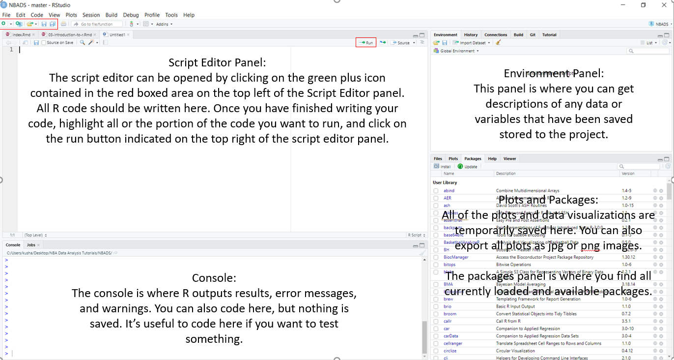
When you open RStudio, this is what you see. Take a look at Figure 1 below to get a brief idea about what the main purpose of the big three panels are. Figure 1:Interface

3.5 Calculation with $\texttt{R}$

Before starting to learn about data analysis, we should learn about how to use $\texttt{R}$ for basic calculations. You can perform all of the basic mathematical operations with $\texttt{(+, -, *, / or ^)}$ as shown below.

2 + 2

## [1] 4

3 - 7

## [1] -4

12*2

## [1] 24

13/2

## [1] 6.5

6^2

## [1] 36

If a particular number will be used often, you can store it into a variable with the assignment operator $\texttt{<-}$. The name of the variable is written on the left and the information you want to save is written on the right side of the assignment operator. All variables that you create are stored in memory. You can look at all of the different variables and their values in the environment panel. You can print the values of the variables in the console by simply typing its name either in the script editor or the console.

pi <- 3.14
r <- 2
area <- pi*r^2
area

## [1] 12.56

3.5.1 Vectors

The one specific design choice that makes $\texttt{R}$ so good for data analysis is the vector data type. A vector in $\texttt{R}$ is a ordered sequence of data elements all of the same type. The numbers that we wrote above have a data type of numeric. All vectors are created with the concatenate function $\texttt{c()}$. If two or more vectors are of the same type, you can perform mathematical operations on them. The mathematical operations are performed element-wise. You can even apply appropriate built in $\texttt{R}$ functions on the vector. Let’s create a numeric vector and do some examples.

x <- c(1,2,3,4,5)
y <- c(6,7,8,9,10)
x

## [1] 1 2 3 4 5

sum(x)

## [1] 15

mean(x)

## [1] 3

var(y)

## [1] 2.5

x + y

## [1]  7  9 11 13 15

x^y

## [1]       1     128    6561  262144 9765625

y^x

## [1]      6     49    512   6561 100000

Another important type of data type is the string, which is treated like text. String data types are initiated by surrounding the individual text that you type with quotes.

message1 <- c("I am", "learning how to use", "R")
message1

## [1] "I am"                "learning how to use" "R"

3.5.2 Logical Operators

A logical operator is an operator that tells you whether a particular statement is true of false. In $\texttt{R}$, we have nine logical operators that will be used frequently:$\texttt{>,>=,<,<=,==,!=,|,&}$. The output of a logical operator is either $TRUE$ or $FALSE$. Let $a$ and $b$ be numbers, and let $x$ and $y$ be declarative statements. The logical operators below have the following meanings:

$a > b$: Is $a$ greater than $b$
$a >= b$: Is $a$ greater or equal to $b$?
$a < b$: Is $a$ less than $b$?
$a <= b$: Is $a$ less than or equal to $b$?
$a == b$: Is $a$ equal to $b$?
$x != y$: Is $a$ NOT equal to $b$?
$x|y$: If at least on of the following statements are true, $\texttt{TRUE}$ is outputted, $x$, $y$, or $x$ and $y$
$x\&y$: Both $x$ and $y$ have to true in order for the output to be $TRUE$.

Logical operators are performed element wise on vectors. Let’s do some examples.

5 > 4

## [1] TRUE

4 > 5

## [1] FALSE

(4 + 7) == (18 - 7)

## [1] TRUE

((4 + 7) == (18 - 7))|(3 > 5) # Make sure you understand the difference between this and the next one

## [1] TRUE

((4 + 7) == (18 - 7))&(3 > 5)

## [1] FALSE

c(1,3,5,7,9,11) > 4

## [1] FALSE FALSE  TRUE  TRUE  TRUE  TRUE

3.5.3 Functions

We have already seen some functions above, such as $\texttt{c()}$, $\texttt{sum()}$, $\texttt{mean()}$, and $\texttt{var()}$. $\texttt{R}$ functions are similar to the functions that you have learned in algebra. A function takes in one or more arguements, and spits out an output. There are many functions in $\texttt{R}$, way too many to detail all of them. We will learn about many $\texttt{R}$ functions as they become relevant. But for now, let’s analyze a specific function $\texttt{seq()}$ to learn about how functions work in general.

The $\texttt{seq()}$ functions creates a numeric vector that contains a sequence of incremented numbers. Every $\texttt{R}$ function has inputs that you have to provide. For the $\texttt{seq()}$ function, the general inputs are \[ \texttt{seq(from = STARTING NUMBER, to = ENDING NUMBER, by = INCREMENT).}\] The inputs $\texttt{from}$, $\texttt{to}$, and $\texttt{by}$ don’t have to be in order, but you do have to specify which input you’re making. A function can also have inputs that are optional. For example, $\texttt{length.out}$ specifies how many numbers you want in your sequence. Let’s do an example by creating a sequence that starts from 1, ends at 2, and increases by 0.1.

my_seq <- seq(from = 1, to = 2, by = 0.1)
my_seq

##  [1] 1.0 1.1 1.2 1.3 1.4 1.5 1.6 1.7 1.8 1.9 2.0

What if you’re not sure how a function works? You can either search for the documentation on the function by either searching for it in the help panel which is located next to the plots and packages panel, or type $\texttt{?function}$ into the console, where $\texttt{function}$ is the name of the function you want to learn about. For example, if you wanted to learn about the covariance function $\texttt{cov()}$, you type $\texttt{?cov}$ into the console. Another option is search for the function on google, where you may find alternative documentation and examples about how a particular function works.

3.6 NBA Data

Let’s finally get to working with NBA data! As I mentioned before, you can download a library called $\texttt{nbastatR}$, which can load a ridiculous amount of historical and current NBA data into $\texttt{R}$ for you. The $\texttt{nbastatR}$ was created by $\texttt{R}$ enthusiast Alex Bresler. The $\texttt{nbastatR}$ library contains numerous amounts of data such as player level data, team level data, injuries, draft data, NBA combine data, and much more! This library will be our main source for NBA data throughout the tutorials, but other sources for NBA data will also discussed briefly.

To install $\texttt{nbastatR}$, or any library for that matter, you simply type $\texttt{install.packages("nbastatR")}$ to install the library and $\texttt{library("nbastatR")}$ to load it in. Notice that the name of the library has to surrounded by quotes. In preparation for stuff to come , download and install the $\texttt{tidyverse}$ package.

library("nbastatR")
library("tidyverse")

After you have installed and loaded these libraries,type $\texttt{nbastatR}$ into the search bar of the packages panel and click on the link. This is the documentation for the $\texttt{nbastatR}$ package. In the documentation, you can find information about what functions are available to use through the library. A majority of these functions are used to load NBA data from various sources into $\texttt{R}$. I recommend taking a quick look at what types of NBA data is available to use.

We will explore the $\texttt{tidyverse}$ and $\texttt{nbastatR}$ libraries extensively throughout these tutorials, but for now, lets load per game and totals NBA data for the 2008 to 2010 seasons by using the $\texttt{bref_players_stats()}$ function. There are many inputs into this function, but we only need to specify information for the $\texttt{seasons}$ and the $\texttt{tables}$ inputs. You can (and should) take a look the documentation about this function to get a better idea about what type of data you can access with it. Once you have loaded the data with this function, a useful function to take a quick look at the first few columns and rows of your data is the $\texttt{head()}$ function.

# Loading season data
NBAData <- bref_players_stats(seasons = 2008:2010, tables = c( "per_game","totals"))

## parsed http://www.basketball-reference.com/leagues/NBA_2008_per_game.html
## parsed http://www.basketball-reference.com/leagues/NBA_2009_per_game.html
## parsed http://www.basketball-reference.com/leagues/NBA_2010_per_game.html
## parsed http://www.basketball-reference.com/leagues/NBA_2008_totals.html
## parsed http://www.basketball-reference.com/leagues/NBA_2009_totals.html
## parsed http://www.basketball-reference.com/leagues/NBA_2010_totals.html
## PerGame
## Totals

head(NBAData)

## # A tibble: 6 x 64
##   slugSeason namePlayer groupPosition yearSeason slugPosition isSeasonCurrent
##   <chr>      <chr>      <chr>              <dbl> <chr>        <lgl>          
## 1 2007-08    Shareef A… F                   2008 PF           FALSE          
## 2 2007-08    Arron Aff… G                   2008 SG           FALSE          
## 3 2007-08    Maurice A… G                   2008 SG           FALSE          
## 4 2007-08    Blake Ahe… G                   2008 PG           FALSE          
## 5 2007-08    LaMarcus … F                   2008 PF           FALSE          
## 6 2007-08    Malik All… F                   2008 PF           FALSE          
## # … with 58 more variables: slugPlayerSeason <chr>, slugPlayerBREF <chr>,
## #   agePlayer <dbl>, slugTeamBREF <chr>, countGames <dbl>,
## #   countGamesStarted <dbl>, pctFG <dbl>, pctFG3 <dbl>, pctFG2 <dbl>,
## #   pctEFG <dbl>, pctFT <dbl>, isHOFPlayer <lgl>, slugTeamsBREF <chr>,
## #   idPlayerNBA <dbl>, urlPlayerThumbnail <chr>, urlPlayerHeadshot <chr>,
## #   urlPlayerPhoto <chr>, urlPlayerStats <chr>, urlPlayerActionPhoto <chr>,
## #   minutesPerGame <dbl>, fgmPerGame <dbl>, fgaPerGame <dbl>,
## #   fg3mPerGame <dbl>, fg3aPerGame <dbl>, fg2mPerGame <dbl>, fg2aPerGame <dbl>,
## #   ftmPerGame <dbl>, ftaPerGame <dbl>, orbPerGame <dbl>, drbPerGame <dbl>,
## #   trbPerGame <dbl>, astPerGame <dbl>, stlPerGame <dbl>, blkPerGame <dbl>,
## #   tovPerGame <dbl>, pfPerGame <dbl>, ptsPerGame <dbl>,
## #   countTeamsPlayerSeasonPerGame <dbl>, minutesTotals <dbl>, fgmTotals <dbl>,
## #   fgaTotals <dbl>, fg3mTotals <dbl>, fg3aTotals <dbl>, fg2mTotals <dbl>,
## #   fg2aTotals <dbl>, ftmTotals <dbl>, ftaTotals <dbl>, orbTotals <dbl>,
## #   drbTotals <dbl>, trbTotals <dbl>, astTotals <dbl>, stlTotals <dbl>,
## #   blkTotals <dbl>, tovTotals <dbl>, pfTotals <dbl>, ptsTotals <dbl>,
## #   countTeamsPlayerSeasonTotals <dbl>, urlPlayerBREF <chr>

I stored this data into a variable called $\texttt{NBAData}$ and will appear in your environment panel. Note that we have assigned an entire dataset into the $\texttt{NBAData}$ variable. This variable has the data type tibble, which is an oddly named data type that includes the traditional rows and columns structure of a dataset. The $\texttt{head(NBAData)}$ function outputted the first few rows and columns of the data, but you can click on the $\texttt{NBAData}$ button on your environment panel to take a look at all of the rows and columns of the data. You can see that the full dataset that we have loaded has $1338$ observations with $64$ variables.

3.7 Data Analysis with the $\texttt{tidyverse}$

We now have a good introduction to the basics of $\texttt{R}$ and a large source of NBA data to start getting into data analysis. As I hinted at in the beginning of this section, we will use a $\texttt{R}$ library called $\texttt{tidyverse}$ to work with data. The $\texttt{tidyverse}$ is a collection of packages developed by Hadley Wickham that aim to create a more efficient framework for data analysis. The $\texttt{tidyverse}$ package is comprised of eight other packages. The most important ones that we will use are,

$\texttt{readr}$: A package that introduces several functions that makes importing data into $\texttt{R}$ more efficient
$\texttt{tidy}$: A package that introduces data types and functions that are meant to convert your data into a certain format. For our purposes, the $\texttt{nbastatR}$ loads our data in a very clean format, so this package won’t be a major area of focus.
$\texttt{dplyr}$: This package is one of the most important for data analysis in $\texttt{R}$. Compared to base $\texttt{R}$, this $\texttt{dplyr}$ will allow us to write and read code that is easier to interpret. We will use this package extensivley throughout these tutorials.
$\texttt{ggplot2}$: Also another important package. This will be our main source of functions and data types for data visualization. An entire section will be devoted to exploring $\texttt{ggplot2}$. For this part of the tutorial, you should download and install the $\texttt{tidyverse}$ package.

3.7.1 Importing Data

Let’s briefly discuss some useful functions from the $\texttt{readr}$ package. We have a ton of data available from the $\texttt{nbastatR}$ package, but what if you have other interesting data? A very interesting type of NBA data is play by play data (PBP). Unfortunately, PBP data is very hard to come by for us fans and is not available on $\texttt{nbastatR}$. PBP data starting from the 1996 season is available online at $\texttt{bigdataball.com}$, but they’ll make sure to rob you of a big chunk of change first. Alternatively, a quick google search will show you that Kaggle user schmadamco has somehow sourced and made available PBP data starting from 2015 to 2021. You can find it on the link here $\texttt{https://www.kaggle.com/schmadam97/nba-playbyplay-data-20182019}$. In fact, Kaggle is great way to find data for almost everything, including other types of sports data. Kaggle also has data science competitions where you can evaluate your data skills. I encourage you to explore Kaggle and try to find data and competitions that interest you.

Let’s learn how to load this data into $\texttt{R}$. Download the data from the link to Kaggle provided above. First of all, the file for your data has to placed in the same location as your current $\texttt{R}$ working directory , the folder path where the $\texttt{R}$ script that you’re working on is located. If you don’t know where this is, you can retrieve it by using the $\texttt{getwd()}$ function (no inputs are needed). Let’s load the 2015 - 2016 PBP data into our environment.

PBP15 <- read_csv(file = "NBA_PBP_2015-16.csv")

This is how you should load data files the with csv file extension type into $\texttt{R}$. Another common file type for data are xls or xlsx files for Microsoft Excel. To load these files into $\texttt{R}$, you have two options. One method is to load the excel file into Microsoft Excel and then export the data as a csv file. Then you can use the $\texttt{read_csv()}$ function to load the data into $\texttt{R}$ as usual. The second option is to download the $\texttt{readxl}$ library and use the $\texttt{read_excel()}$ function as you would with the $\texttt{read_csv()}$ function.

3.7.2 Data Wrangling with $\texttt{dplyr}$

One of the most important and boring aspects of data analysis is data wrangling, the process of gathering, selecting, and transforming data. Unfortunately, if you’re working with raw or fresh data, data wrangling will probably comprise more than $50\%$ of your time spent on a data science project. Luckily for us, $\texttt{nbastatR}$ imports very clean data for us! In most cases we can skip the data cleaning process and get to the fun stuff like data visualization and modeling. However, there are many situations where we still need to transform and filter the data to get better insights about our data and create better measurements. If you are following these tutorials with Python, I recommend using the pandas library for data wrangling.

Understanding $\texttt{dplyr}$ means understanding five verbs (functions): $\texttt{mutate()} , \texttt{select()}, \texttt{filter()}, \texttt{summarise()},$ and $\texttt{arrange()}$. These are the main five functions that you will use for data wrangling with the occasional use of $\texttt{group_by()}$. Earlier, we loaded per game data for the 2008 to 2010 NBA seasons. We will use this dataset throughout the data wrangling tutorials. This data mostly includes mostly average box score measurements, not advanced stats. We actually could have included the advanced stats, but I left them out on purpose to give some motivating examples for data wrangling.

The $\texttt{filter()}$ command allows you to show only those rows your data that obey some condition. Suppose we wanted to identify the players across the 2008 to 2010 seasons that score more than 27 points per game. With the $\texttt{filter()}$ command, we input the name of the data set as the first argument, and the logical statement in the second argument.

filter(NBAData, ptsPerGame > 27)

## # A tibble: 7 x 64
##   slugSeason namePlayer groupPosition yearSeason slugPosition isSeasonCurrent
##   <chr>      <chr>      <chr>              <dbl> <chr>        <lgl>          
## 1 2007-08    Kobe Brya… G                   2008 SG           FALSE          
## 2 2007-08    LeBron Ja… F                   2008 SF           FALSE          
## 3 2008-09    LeBron Ja… F                   2009 SF           FALSE          
## 4 2008-09    Dwyane Wa… G                   2009 SG           FALSE          
## 5 2009-10    Carmelo A… F                   2010 SF           FALSE          
## 6 2009-10    Kevin Dur… F                   2010 SF           FALSE          
## 7 2009-10    LeBron Ja… F                   2010 SF           FALSE          
## # … with 58 more variables: slugPlayerSeason <chr>, slugPlayerBREF <chr>,
## #   agePlayer <dbl>, slugTeamBREF <chr>, countGames <dbl>,
## #   countGamesStarted <dbl>, pctFG <dbl>, pctFG3 <dbl>, pctFG2 <dbl>,
## #   pctEFG <dbl>, pctFT <dbl>, isHOFPlayer <lgl>, slugTeamsBREF <chr>,
## #   idPlayerNBA <dbl>, urlPlayerThumbnail <chr>, urlPlayerHeadshot <chr>,
## #   urlPlayerPhoto <chr>, urlPlayerStats <chr>, urlPlayerActionPhoto <chr>,
## #   minutesPerGame <dbl>, fgmPerGame <dbl>, fgaPerGame <dbl>,
## #   fg3mPerGame <dbl>, fg3aPerGame <dbl>, fg2mPerGame <dbl>, fg2aPerGame <dbl>,
## #   ftmPerGame <dbl>, ftaPerGame <dbl>, orbPerGame <dbl>, drbPerGame <dbl>,
## #   trbPerGame <dbl>, astPerGame <dbl>, stlPerGame <dbl>, blkPerGame <dbl>,
## #   tovPerGame <dbl>, pfPerGame <dbl>, ptsPerGame <dbl>,
## #   countTeamsPlayerSeasonPerGame <dbl>, minutesTotals <dbl>, fgmTotals <dbl>,
## #   fgaTotals <dbl>, fg3mTotals <dbl>, fg3aTotals <dbl>, fg2mTotals <dbl>,
## #   fg2aTotals <dbl>, ftmTotals <dbl>, ftaTotals <dbl>, orbTotals <dbl>,
## #   drbTotals <dbl>, trbTotals <dbl>, astTotals <dbl>, stlTotals <dbl>,
## #   blkTotals <dbl>, tovTotals <dbl>, pfTotals <dbl>, ptsTotals <dbl>,
## #   countTeamsPlayerSeasonTotals <dbl>, urlPlayerBREF <chr>

We can make more complex filters too. For example, we can find the players that had more than 27 points per game or less than 15 points per game, while averaging more than 8 assists per game.

filter(NBAData, ptsPerGame > 27 | ptsPerGame < 15, astPerGame > 8)

## # A tibble: 10 x 64
##    slugSeason namePlayer groupPosition yearSeason slugPosition isSeasonCurrent
##    <chr>      <chr>      <chr>              <dbl> <chr>        <lgl>          
##  1 2007-08    Jose Cald… G                   2008 PG           FALSE          
##  2 2007-08    Jason Kidd G                   2008 PG           FALSE          
##  3 2007-08    Jamaal Ti… G                   2008 PG           FALSE          
##  4 2008-09    Gilbert A… G                   2009 PG           FALSE          
##  5 2008-09    Jose Cald… G                   2009 PG           FALSE          
##  6 2008-09    Jason Kidd G                   2009 PG           FALSE          
##  7 2008-09    Rajon Ron… G                   2009 PG           FALSE          
##  8 2009-10    LeBron Ja… F                   2010 SF           FALSE          
##  9 2009-10    Jason Kidd G                   2010 PG           FALSE          
## 10 2009-10    Rajon Ron… G                   2010 PG           FALSE          
## # … with 58 more variables: slugPlayerSeason <chr>, slugPlayerBREF <chr>,
## #   agePlayer <dbl>, slugTeamBREF <chr>, countGames <dbl>,
## #   countGamesStarted <dbl>, pctFG <dbl>, pctFG3 <dbl>, pctFG2 <dbl>,
## #   pctEFG <dbl>, pctFT <dbl>, isHOFPlayer <lgl>, slugTeamsBREF <chr>,
## #   idPlayerNBA <dbl>, urlPlayerThumbnail <chr>, urlPlayerHeadshot <chr>,
## #   urlPlayerPhoto <chr>, urlPlayerStats <chr>, urlPlayerActionPhoto <chr>,
## #   minutesPerGame <dbl>, fgmPerGame <dbl>, fgaPerGame <dbl>,
## #   fg3mPerGame <dbl>, fg3aPerGame <dbl>, fg2mPerGame <dbl>, fg2aPerGame <dbl>,
## #   ftmPerGame <dbl>, ftaPerGame <dbl>, orbPerGame <dbl>, drbPerGame <dbl>,
## #   trbPerGame <dbl>, astPerGame <dbl>, stlPerGame <dbl>, blkPerGame <dbl>,
## #   tovPerGame <dbl>, pfPerGame <dbl>, ptsPerGame <dbl>,
## #   countTeamsPlayerSeasonPerGame <dbl>, minutesTotals <dbl>, fgmTotals <dbl>,
## #   fgaTotals <dbl>, fg3mTotals <dbl>, fg3aTotals <dbl>, fg2mTotals <dbl>,
## #   fg2aTotals <dbl>, ftmTotals <dbl>, ftaTotals <dbl>, orbTotals <dbl>,
## #   drbTotals <dbl>, trbTotals <dbl>, astTotals <dbl>, stlTotals <dbl>,
## #   blkTotals <dbl>, tovTotals <dbl>, pfTotals <dbl>, ptsTotals <dbl>,
## #   countTeamsPlayerSeasonTotals <dbl>, urlPlayerBREF <chr>

The two statements above tried to print way too much information than what could fit onto the screen, hence those annoying comments. What if we wanted to limit the numbers of columns that are printed? If we’re filtering by points and assists, we probably wouldn’t care about other information. To do this, we use the $\texttt{select()}$ function. Input the name of the dataset or the filter as the first arguement and the names of the columns that you want to keep on the other arguements.

select(filter(NBAData,ptsPerGame > 27 | ptsPerGame < 15, astPerGame > 8), namePlayer,ptsPerGame,astPerGame,slugSeason)

## # A tibble: 10 x 4
##    namePlayer     ptsPerGame astPerGame slugSeason
##    <chr>               <dbl>      <dbl> <chr>     
##  1 Jose Calderon        11.2        8.3 2007-08   
##  2 Jason Kidd           10.8       10.1 2007-08   
##  3 Jamaal Tinsley       11.9        8.4 2007-08   
##  4 Gilbert Arenas       13         10   2008-09   
##  5 Jose Calderon        12.8        8.9 2008-09   
##  6 Jason Kidd            9          8.7 2008-09   
##  7 Rajon Rondo          11.9        8.2 2008-09   
##  8 LeBron James         29.7        8.6 2009-10   
##  9 Jason Kidd           10.3        9.1 2009-10   
## 10 Rajon Rondo          13.7        9.8 2009-10

That code that we just wrote had a lot of parenthesis. This makes it harder to read and interpret. For this reason, we introduce the pipe operator $\texttt{ %>% }$. The piper operator will be typed a lot, so a shortcut is handy. By default you type $\texttt{Ctrl + Shift + M}$ (Windows) or $\texttt{Cmd + Shift + M}$ (Mac) to type it automatically. The pipe operator takes a value on the left side of the symbol, and inputs that value into the first arguement of the function that is typed on the right side of the symbol.An example will make more sense.

NBAData %>% filter(ptsPerGame > 27 | ptsPerGame < 15,astPerGame > 8) %>% 
  select(namePlayer,ptsPerGame,astPerGame,slugSeason)

## # A tibble: 10 x 4
##    namePlayer     ptsPerGame astPerGame slugSeason
##    <chr>               <dbl>      <dbl> <chr>     
##  1 Jose Calderon        11.2        8.3 2007-08   
##  2 Jason Kidd           10.8       10.1 2007-08   
##  3 Jamaal Tinsley       11.9        8.4 2007-08   
##  4 Gilbert Arenas       13         10   2008-09   
##  5 Jose Calderon        12.8        8.9 2008-09   
##  6 Jason Kidd            9          8.7 2008-09   
##  7 Rajon Rondo          11.9        8.2 2008-09   
##  8 LeBron James         29.7        8.6 2009-10   
##  9 Jason Kidd           10.3        9.1 2009-10   
## 10 Rajon Rondo          13.7        9.8 2009-10

You don’t have to separate each pipe by lines but I find that it makes code more readable. You can try to kind of convert this code into English to have it make more sense. Read the pipe operator as “then”. We can read the code as “Filter NBA Data for points per game greater than 27 or less than 15, and more than 8 assists per game, THEN select the name of the player, points scored per game, assists per game, and the season”. Let’s do one more example for the $\texttt{select()}$ function. Suppose we wanted all of the rows, but only the name of the player, the season played, and all of the columns between and including $\texttt{astPerGame}$ and $\texttt{ptsPerGame}$. Instead of typing all of those columns, we can use $\texttt{astPerGame:ptsPerGame}$ as one input.

NBAData %>% select( namePlayer,slugSeason, astPerGame:ptsPerGame)

## # A tibble: 1,338 x 8
##    namePlayer slugSeason astPerGame stlPerGame blkPerGame tovPerGame pfPerGame
##    <chr>      <chr>           <dbl>      <dbl>      <dbl>      <dbl>     <dbl>
##  1 Shareef A… 2007-08           0.7        0.2        0          0.2       1.5
##  2 Arron Aff… 2007-08           0.7        0.4        0.1        0.5       1.1
##  3 Maurice A… 2007-08           0.3        0          0          0.2       0.7
##  4 Blake Ahe… 2007-08           1.6        0.5        0          1.3       1.7
##  5 LaMarcus … 2007-08           1.6        0.7        1.2        1.7       3.2
##  6 Malik All… 2007-08           0.6        0.3        0.4        0.6       2  
##  7 Ray Allen  2007-08           3.1        0.9        0.2        1.7       2  
##  8 Tony Allen 2007-08           1.5        0.8        0.3        1.5       2.2
##  9 Lance All… 2007-08           0          0          0          0         0.3
## 10 Morris Al… 2007-08           0.3        0.1        0          0.2       0.6
## # … with 1,328 more rows, and 1 more variable: ptsPerGame <dbl>

What if we wanted to find players that scored the least points in the 2009 season in ascending order ? To arrange the rows in a certain order, we can use the $\texttt{arrange()}$ function.

NBAData %>% 
  filter(yearSeason == 2009) %>% 
  select(namePlayer,ptsPerGame) %>% 
  arrange(ptsPerGame)

## # A tibble: 445 x 2
##    namePlayer      ptsPerGame
##    <chr>                <dbl>
##  1 Martell Webster        0  
##  2 Nathan Jawai           0.3
##  3 Mark Madsen            0.3
##  4 Michael Ruffin         0.5
##  5 Sun Sun                0.6
##  6 Joey Dorsey            0.7
##  7 J.R. Giddens           0.7
##  8 Randolph Morris        0.8
##  9 Cheikh Samb            0.8
## 10 Kenny Thomas           0.8
## # … with 435 more rows

Damn. We can also find the players that scored the most points in descending order by adding the $ option.

NBAData %>% 
  filter(yearSeason == 2009) %>% 
  select(namePlayer,ptsPerGame) %>% 
  arrange(desc(ptsPerGame))

## # A tibble: 445 x 2
##    namePlayer      ptsPerGame
##    <chr>                <dbl>
##  1 Dwyane Wade           30.2
##  2 LeBron James          28.4
##  3 Kobe Bryant           26.8
##  4 Dirk Nowitzki         25.9
##  5 Danny Granger         25.8
##  6 Kevin Durant          25.3
##  7 Kevin Martin          24.6
##  8 Al Jefferson          23.1
##  9 Carmelo Anthony       22.8
## 10 Chris Paul            22.8
## # … with 435 more rows

As I mentioned before, I left out the advanced stats to showcase data wrangling examples. We now use the $\texttt{mutate()}$ function to create new columns. Let’s calculate True Shooting Percentage ($TS\%$) for each player. True shooting percentage has the following definition, \[ TS\% = \frac{PTS}{FGA + 0.44FTA}\] Let’s create the $TS\%$ stat, store it into our $\texttt{NBAData}$ data variable, and showcase players arranged by the highest points per game. We can use the $texttt{round()}$ function so less decimals show up in the calculation.

NBAData <- NBAData %>% 
  mutate(TS = round(ptsTotals/(2*(fgaTotals + 0.44*ftaTotals)),3))

NBAData %>% select(namePlayer, ptsPerGame, TS,yearSeason) %>% 
  arrange(desc(ptsPerGame))

## # A tibble: 1,338 x 4
##    namePlayer      ptsPerGame    TS yearSeason
##    <chr>                <dbl> <dbl>      <dbl>
##  1 Dwyane Wade           30.2 0.574       2009
##  2 Kevin Durant          30.1 0.607       2010
##  3 LeBron James          30   0.568       2008
##  4 LeBron James          29.7 0.604       2010
##  5 LeBron James          28.4 0.591       2009
##  6 Kobe Bryant           28.3 0.576       2008
##  7 Carmelo Anthony       28.2 0.548       2010
##  8 Kobe Bryant           27   0.545       2010
##  9 Kobe Bryant           26.8 0.561       2009
## 10 Dwyane Wade           26.6 0.562       2010
## # … with 1,328 more rows

A very important part of NBA analytics is contextualizing the data. For example, shooting efficiency has changed from era to era. We see that Dwayne Wade had a $TS\%$ of $0.574$, but how good was this relative to league average? If you want to calculate the average $TS\%$ for each of the 2008, 2009, and 2010 seasons, we can use the $\texttt{group_by()}$ and $\texttt{summarise()}$ functions to do it quickly.

NBAData %>% 
  group_by(yearSeason) %>% 
  summarise(LgAvgTS = mean(TS,na.rm = TRUE))

## `summarise()` ungrouping output (override with `.groups` argument)

## # A tibble: 3 x 2
##   yearSeason LgAvgTS
##        <dbl>   <dbl>
## 1       2008   0.513
## 2       2009   0.521
## 3       2010   0.525

This creates a separate table of grouped averages. To calculate the relative true shooting percentage for each player, we have to use $\texttt{mutate()$ instead of $\texttt{summarise()$. Let’s calculate relative true shooting for each player for all three seasons.

NBAData <- NBAData %>% 
  group_by(yearSeason) %>% 
  mutate(LgAvgTS = mean(TS,na.rm = TRUE),RelTS = TS - LgAvgTS)

NBAData %>% 
  select(namePlayer,RelTS) %>% 
  arrange(desc(RelTS))

## Adding missing grouping variables: `yearSeason`

## # A tibble: 1,338 x 3
## # Groups:   yearSeason [3]
##    yearSeason namePlayer      RelTS
##         <dbl> <chr>           <dbl>
##  1       2008 Jerome James    0.551
##  2       2010 Ryan Bowen      0.539
##  3       2009 Steven Hill     0.479
##  4       2009 Marcus Williams 0.479
##  5       2010 Trey Gilder     0.475
##  6       2008 Jelani McCoy    0.285
##  7       2009 Eddie Gill      0.257
##  8       2009 Eddy Curry      0.232
##  9       2009 Mouhamed Sene   0.225
## 10       2008 Cheikh Samb     0.204
## # … with 1,328 more rows

3.8 General comments about writing code

In some of the $\texttt{R}$ code blocks there was a hashtag $\texttt{#}$ symbol. When you start a line of code in the script editor with $\texttt{#}$, it tells $\texttt{R}$ to ignore everything on that line. These lines of text that are ignored are referred to as comments. It is good habit to add comments judiciously throughout your code. It is very easy to write a lot of code, walk away from $\texttt{R}$ for a couple of days, and forget what your code is supposed to do. Add comments to give yourself and other people that may read your code some notes about what your code is actually doing.

There are too many functions and intricacies in $\texttt{R}$ to know everything. Read the documentation and google any questions that you may encounter. It’s more important to understand good coding habits rather than memorizing a bunch of syntax.

Data Science and Econometrics for NBA Analytics

Chapter 3 Introduction to \(\texttt{R}\)

3.1 Why \(\texttt{R}\) ?

3.2 What if I want to use Python ?

3.3 How to Install \(\texttt{R}\)