Chapter 2 Examples

2.1 Example 1 - Backward Elimination and Forward Selection

Create regression models for predicting wrestlers’ hydrostatic fat (hwfat) using the data frame HSWRESTLER.

The dataset can be found in the R package PASWR2, which can be loaded in using

library(PASWR2)

1. Perform quality checks on the data in HSWRESTLER as well as some basic exploratory analysis to see how the predictors (age, ht, wt, abs, triceps, and subscap) are related to hwfat.

Consider using the pairs() function to perform preliminary analysis of how the predictors relate to hwfat, as well as the cor() function.

Since we are only interested in the predictors listed in the question, we can remove the last two.

HSWRESTLER <- HSWRESTLER[,-c(8:9)]

pairs(HSWRESTLER)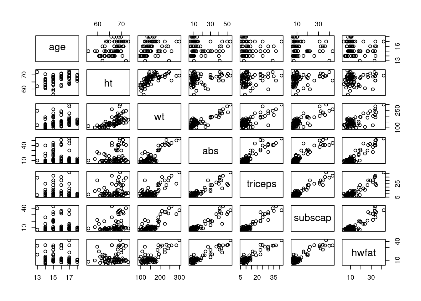

The predictors that appear to best relate to hwfat are wt, abs, triceps and subscap.

cor(HSWRESTLER)

##                 age        ht        wt         abs    triceps    subscap
## age      1.00000000 0.4177471 0.2406721 -0.05970301 -0.1349368 -0.1077762
## ht       0.41774714 1.0000000 0.6044705  0.25882739  0.1578298  0.2525007
## wt       0.24067211 0.6044705 1.0000000  0.84808755  0.7526595  0.8149226
## abs     -0.05970301 0.2588274 0.8480876  1.00000000  0.9057768  0.9254833
## triceps -0.13493683 0.1578298 0.7526595  0.90577680  1.0000000  0.9455530
## subscap -0.10777616 0.2525007 0.8149226  0.92548332  0.9455530  1.0000000
## hwfat   -0.17053777 0.1399135 0.7334894  0.91813556  0.9166337  0.9059425
##              hwfat
## age     -0.1705378
## ht       0.1399135
## wt       0.7334894
## abs      0.9181356
## triceps  0.9166337
## subscap  0.9059425
## hwfat    1.0000000

The correlations back up the initial interpretation, with wt having a slightly weaker linear relationship than the others.

The package car has several useful functions, and the function scatterplotMatrix() may be useful for exploring relationships among the predictors and hwfat. There are a number of arguments/options for the function scatterplotMatrix(), so it's advised to refer to its help page for further details.

library(car)
scatterplotMatrix(x = HSWRESTLER)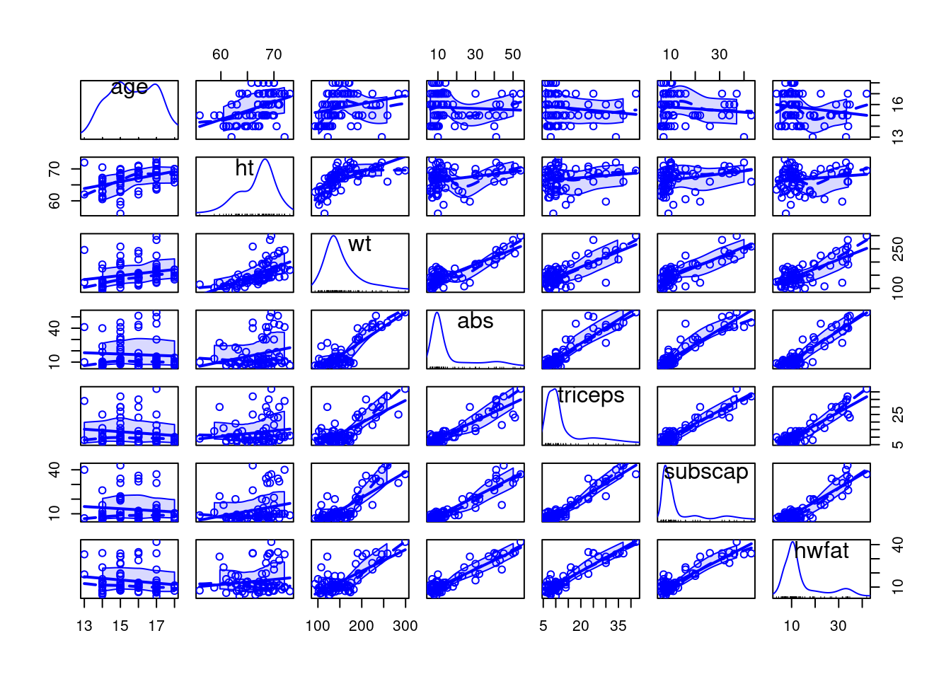

#or 

scatterplotMatrix(formula = ~ hwfat + age + ht + wt + abs + triceps +
+ subscap, data = HSWRESTLER)

The plots generated by scatterplotMatrix() display with more clarity why wt doesn't follow as linear a relationship as the other predictors mentioned above.

2. Use backward elimination with the predictors age, ht, wt, abs, triceps, and subscap and an \(\alpha_{crit}\) of 0.20 to create a regression model where hwfat is the response variable.

Start by defining the full model, with all listed predictors. Then use the function drop1() with a test="F" argument to find the first term to remove based on highest (least significant) p-value.

model.all <- lm(hwfat ~ ., data = HSWRESTLER)

drop1(model.all, test = "F") # single term deletions

## Single term deletions
## 
## Model:
## hwfat ~ age + ht + wt + abs + triceps + subscap
##         Df Sum of Sq    RSS    AIC F value    Pr(>F)    
## <none>               651.05 179.51                      
## age      1     9.594 660.64 178.65  1.0463  0.309839    
## ht       1     1.613 652.66 177.70  0.1759  0.676225    
## wt       1     2.546 653.60 177.81  0.2777  0.599879    
## abs      1   162.000 813.05 194.84 17.6669 7.549e-05 ***
## triceps  1    72.683 723.73 185.76  7.9264  0.006301 ** 
## subscap  1     5.921 656.97 178.21  0.6458  0.424315    
## ---
## Signif. codes:  0 '***' 0.001 '**' 0.01 '*' 0.05 '.' 0.1 ' ' 1

Since the largest p-value from drop1() is 0.6762, which corresponds to the variable ht, one needs to update the original model by dropping the variable ht. The function update() allows the user to update a previous model (model.all) using the short-hand notation. ~ . -ht. The periods on the left and right side of the tilde tell R to use what is specified in the left- and right-hand sides of the tilde in model.all minus the variable ht.

model.new <- update(model.all, . ~ . - ht)

The first variable we remove is noneagehtwtabstricepssubscap

The second variable to be removed is none agehtwtabstricepssubscap

The third variable dropped is noneagehtwtabstricepssubscap

The fourth variable dropped is noneagehtwtabstricepssubscap

3. Use forward selection with the predictors age, ht, wt, abs, triceps, and subscap and an \(\alpha_{crit}\) of 0.20 to create a regression model where hwfat is the response variable.

The functions add1() and update() are used to create a model using forward selection.

SCOPE <- (~ . + age + ht + wt + abs + triceps + subscap)

mod.fs <- lm(hwfat ~ 1, data = HSWRESTLER) # create a new empty model for Forwards Selection

add1(mod.fs, scope = SCOPE, test = "F") # SCOPE defined above determines the variables to be added

## Single term additions
## 
## Model:
## hwfat ~ 1
##         Df Sum of Sq    RSS    AIC  F value    Pr(>F)    
## <none>               6017.8 340.97                       
## age      1     175.0 5842.8 340.67   2.2765    0.1355    
## ht       1     117.8 5900.0 341.43   1.5175    0.2218    
## wt       1    3237.6 2780.2 282.74  88.5045 2.219e-14 ***
## abs      1    5072.8  945.0 198.57 407.9929 < 2.2e-16 ***
## triceps  1    5056.3  961.5 199.92 399.6462 < 2.2e-16 ***
## subscap  1    4939.0 1078.8 208.90 347.9456 < 2.2e-16 ***
## ---
## Signif. codes:  0 '***' 0.001 '**' 0.01 '*' 0.05 '.' 0.1 ' ' 1

mod.fs <- update(mod.fs, . ~ . + abs)

We look to add the term which results in the lowest AIC for the model, since multiple variables are below the \(\alpha_{crit}\) of 0.20.

The first variable we add is noneagehtwtabstricepssubscap

The second variable to be added is none agehtwtabstricepssubscap

The third variable added is noneagehtwtabstricepssubscap

The third variable added is noneagehtwtabstricepssubscap