3.2 Weighted log odds ratio
This section is heavily based on Monroe, Colaresi, and Quinn(2008) and a medium post, titled I dare say you will never use tf-idf again.
3.2.1 Log odds ratio
First, the log odds of word \(w\) in document \(i\) is defined as
\[ \log{O_{w}^i} = \log{\frac{f_w^i}{1 - f_w^i}} \]
Logging the odds ratio provides a measure that is symmetric when comparing the usage of word \(w\) across different documents. Log odds ratio of word \(w\) between document \(i\) and \(j\) is
\[ \log{\frac{O_{w}^i}{O_w^j}} = \log{\frac{f_w^i}{1 - f_w^i} / \frac{f_w^j}{1 - f_w^j}} = \log{\frac{f_w^i}{1 - f_w^i}} - log{\frac{f_w^j}{1 - f_w^j}} \] A problem is that, when some word \(w\) is only presented in document \(i\), among other documents in the corpus, odds ratio will have zero denominator and the metric goes to infinity. One solution is to “add a little bit to the zeroes”, in which smoothed word frequency is defined as \(\tilde{f_w^i} = f_w^i + \varepsilon\).
Note that regardless of the zero treatment, words with hightest log odds ratio are often obscure ones. The problem is again the failure to account for sampling variability. With logodds ratios, the sampling variation goes down with increased frequency. So that different words are not comparable.
A common response to this is to set some frequency “threshold” for features to ‘‘qualify’’ for consideration. For example, we only compute log odds ratio on words that appears at least 10 times.
3.2.2 Model-based approach: Weighted log odds ratio
Monroe, Colaresi, and Quinn then proposed a model-basded approach where the choice of word \(w\) are modelled as a function oof document \(P(w |j)\). In general, the strategy is to first model word usage in the full collection of documents and to then investigate how subgroup-specific word usage diverges from that in the full collection of documents.
First, the moel assumes that the W-vector \(\boldsymbol{y}\) follows a multinomial distribution
\[ \boldsymbol{y} \sim \text{Multinomial}(n, \boldsymbol{\pi}) \] where \(n = \sum_{w=1}^Wy_w\) and \(\boldsymbol{\pi}\) is W-vector of possibilities. And the the baseline log odds ratio between word \(w\) and the first word is
\[ \beta_w = \log{\pi_w} - \log{\pi_1} \;\;\; w=1, 2, ..., W \]
BTW, this is essentially a baseline logit model including only an intercept, which is an extention of logistic regression for dealing with response with W categories.
Therefore, the likelihood function can be expressed in terms of \(\beta_w\)
\[ L(\boldsymbol{\beta} | \boldsymbol{y}) = \prod_{w=1}^{W}{(\frac{\exp(\beta_w)}{\sum_{w=1}^{W}\exp(\beta_w)})^{y_w}} \]
Within any document, \(i\), the model to this point goes through with addition of subscripts
\[ \boldsymbol{y^i} \sim \text{Multinomial}(n^i, \boldsymbol{\pi^i}) \]
The lack of covariates results in an immediately available analytical solution for the MLE of \({\beta^i_w}\) . We calculate
\[ \boldsymbol{\hat{\pi}}^\text{MLE} = \boldsymbol{y} / n \]
where \(n = \sum_{w = 1}^{W}y_w\)and \(\boldsymbol{\hat{\beta}}^\text{MLE}\) follows after transforming.
The paper proceeds with a Bayesian model, specifying the prior using the conjugate for the multinomial distribution, the Dirichlet:
\[ \boldsymbol{\pi} \sim \text{Dirichlet}(\boldsymbol{\alpha}) \] where \(\boldsymbol{\alpha}\) is a W-vector of parameters with each element \(\alpha_w > 0\). There is a nice interpretation of \(\alpha_w\), that is, use of any particular Dirichlet prior defined by \(\boldsymbol{\alpha}\) affects the posterior exactly as if we had observed in the data an additional \(\alpha_w – 1\) instances of word \(w\). It follows this is a uninformative prior if all \(\alpha_w\)s are identitcal.
Due to the conjugacy, the full Bayesian estimate using the Dirichlet prior is also analytically available in analogous form:
\[ \boldsymbol{\hat{\pi}} = \frac{(\boldsymbol{y} + \boldsymbol{\alpha})}{n + \alpha_0} \] where \(\alpha_0 = \sum_{w=1}^{W}\alpha_w\)
Our job, therefore, is to compare if the usage of word \(w\) in document \(i\), \(\pi_w^i\), differs from \(\pi_w\) overall or in some other document \(\pi^j_w\). One of the advantages of the model-based approach is that we can measure the uncertainty in odds.
Denote the odds (now with probabilistic meaning) of word w, relative to all others, as \(\Omega_w = \pi_w / (1- \pi_w)\). We are interested in how the usage of a word by document \(i\) differs from usage of the word in all documents, which we can capture with the log-odds-ratio, which we will now define as \(\delta_w^i = \log{\Omega_w^i / \Omega_w}\). To compare between documents \(i\) and \(j\), log odds ratio of word \(w\) is defined as \(\delta_w^{i-j} = \log{\Omega_w^i / \Omega_w^j}\). To scale these two estimators, their point estimate and estimated variance are found
\[ \begin{aligned} \hat{\delta}_{w}^{i-j} &= \log(\frac{y_w^i + \alpha_w}{n^i + \alpha_0 - (y_w^i + \alpha_w)}) - \log(\frac{y_w^j + \alpha_w}{n^j + \alpha_0 - (y_w^j + \alpha_w)}) \\ \sigma^2(\hat{\delta}_{w}^{i-j}) &\approx \frac{1}{y_w^i + a_w} + \frac{1}{y_w^j + a_w} \end{aligned} \] The final standardized statistic for a word \(w\) is then the z–score of its log–odds–ratio:
\[ \frac{\hat{\delta}_{w}^{i-j}}{\sigma^2(\hat{\delta}_{w}^{i-j})} \]
The Monroe, et al method then uses counts from a background corpus to provide a prior count for words, rather than the uninformative Dirichlet prior, essentially shrinking the counts toward to the prior frequency in a large background corpus to prevent overfitting. The general notion is to put a strong conservative prior (regularization) on the model, requiring the data to speak very loudly if such a difference is to be declared. I am not going to dive into that. But it is important to know that \(\alpha_0 = 1\) means no shrinkage, and \(\alpha_0 \rightarrow 0\) or \(\alpha_0 \rightarrow \infty\) mean strongest shrinkage.
3.2.3 Discussions
The Monroe, modifies the commonly used log–odds ratio (introduced in Section 3.2.1) in two ways (Jurafsky et al. 2014) :
It uses the z–scores of the log–odds–ratio, which controls for the amount of variance in a word’s frequency. So the score on different words are comparable. And the metric also faciliates interpretation, positive log odds means stronger tendency to use the word, and negative ones indicate otherwise. Also, \(|\hat{\delta}^i_w| > 1.96\) should mean some sort of significance.
Secondly, it uses counts from a background corpus to provide a prior count for words, essentially shrinking the counts toward to the prior frequency in a large background corpus. These features enable differences even in very frequent words to be detected; previous linguistic methods have all had problems with frequent words. Because function words like pronouns and auxiliary verbs are both extremely frequent and have been shown to be important cues to social and narrative meaning, this is a major limitation of these methods. For example, as an English reader/speaker, you won’t be surprised that all the authors you are trying to compare use “of the” and “said the” in their respective documents, and we want to know who used much more than others. tf-idf will not be able to detect this, because the idf of words appearing in every document will always be zero.
3.2.4 bind_log_odds()
There is an issue suggesting that tidylo is still experimental. However, it did provide a ussful function bind_log_odds() that implemented the weighted log odds we dicussed above, and it seems that it currently uses the marginal distributions (i.e., distribution of words across all documents combined) to construct an informative Dirichlet prior.
The data structure bind_log_odds() requires is the same with bind_tf_idf()
library(tidylo)
book_words %>%
bind_log_odds(set = book, feature = word, n = n) %>%
arrange(desc(log_odds))
#> # A tibble: 40,379 x 7
#> book word n tf idf tf_idf log_odds
#> <fct> <chr> <int> <dbl> <dbl> <dbl> <dbl>
#> 1 Emma emma 786 0.00488 1.10 0.00536 24.5
#> 2 Mansfield Park fanny 816 0.00509 0.693 0.00352 24.1
#> 3 Sense & Sensibility elinor 623 0.00519 1.79 0.00931 23.4
#> 4 Pride & Prejudice elizabeth 597 0.00489 0.693 0.00339 21.0
#> 5 Sense & Sensibility marianne 492 0.00410 1.79 0.00735 20.8
#> 6 Persuasion anne 447 0.00534 0.182 0.000974 20.6
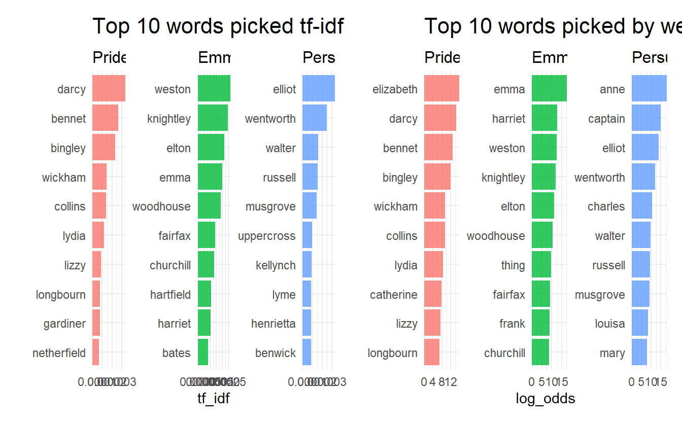
#> # ... with 4.037e+04 more rowsNow let’s compare the result between tf-idf and weighted log odds in a subset of book_words
words_tf_idf <- book_words %>%
  filter(book %in% c("Emma", "Pride & Prejudice", "Persuasion")) %>%
  bind_tf_idf(term = word, document = book, n = n) %>%
  group_by(book) %>%
  top_n(10) %>%
  ungroup() %>%
  facet_bar(y = word, x = tf_idf, by = book, ncol = 3) +
  labs(title = "Top 10 words picked tf-idf")

words_wlo <- book_words %>%
  filter(book %in% c("Emma", "Pride & Prejudice", "Persuasion")) %>%
  bind_log_odds(feature = word, set = book, n = n) %>%
  group_by(book) %>%
  top_n(10) %>%
  ungroup() %>%
  facet_bar(y = word, x = log_odds, by = book, ncol = 3) +
  labs(title = "Top 10 words picked by weighted log odds")