Chapter 2 Using R to Do Data Analysis
One of the important goals of this book is to introduce students to R, a programming language that facilitates data analysis. Hopefully, you will learn enough here to feel comfortable using R to accomplish simple statistical tasks and to move into more advanced uses of R with relative ease. There are many reasons to use R, including that it is free. In addition to being free, R also helps students develop some basic programming skills, keeps them more directly connected to the the data they are using, and encourages them to think a bit more systematically about the problems they are trying to solve. One reason sometimes given for not using R is that there is a steep learning curve. Indeed, there is a bit of a learning curve with R, but this is not a good reason to avoiding R. First, all statistical programs used in courses on data analysis are difficult to learn if students don’t have prior experience with them. Whether using SPSS, Stata, SAS, or even Excel, students with no prior experience will struggle for the first few weeks of the semester. Second, some of the things that make R a bit more difficult to learn at the outset are also the things that provide added value from an educational perspective. Finally, it’s all right for students to be challenged with something that is a bit different from what they are used to. That’s one of the more valuable things about higher learning!
R is used throughout this book to generate virtually all statistical results and graphics. In addition, as an instructional aid, in most cases, the code used to generate graphics and statistical results is provided in the text associated with the results. This sample code can be used by students to solve the R-based problems at the end of the chapters, or as a guide to other problems and homework that might be assigned.
2.1 Accessing R
One important tool that is particularly useful for new users of R is RStudio, a graphical user interface (GUI) that facilitates user\(\rightarrow\)R interactions. If you have reliable access to compute labs on your college or university campus, there’s a good chance that R and RStudio are installed and available for you to use. If so, and if you don’t mind having access only in the labs, then great, there’s no need to download anything. That said, one of the nice things about using R is that you can download it (and RStudio) for free and have instant, anytime access on your own computer.
Downloading and installing R is at once pretty straightforward and at the same time a point in the process where new users encounter a few problems. The first step (#1 in Figure 2.1) is to go to https://www.r-project.org and click on the CRAN (Comprehensive R Archive Network) link on the left side of the web page. This takes you to a collection of local links to CRAN mirrors, arranged by country, from which users can download R. You should select a CRAN that is geographically close to you. (Step 2 in Figure 2.1).
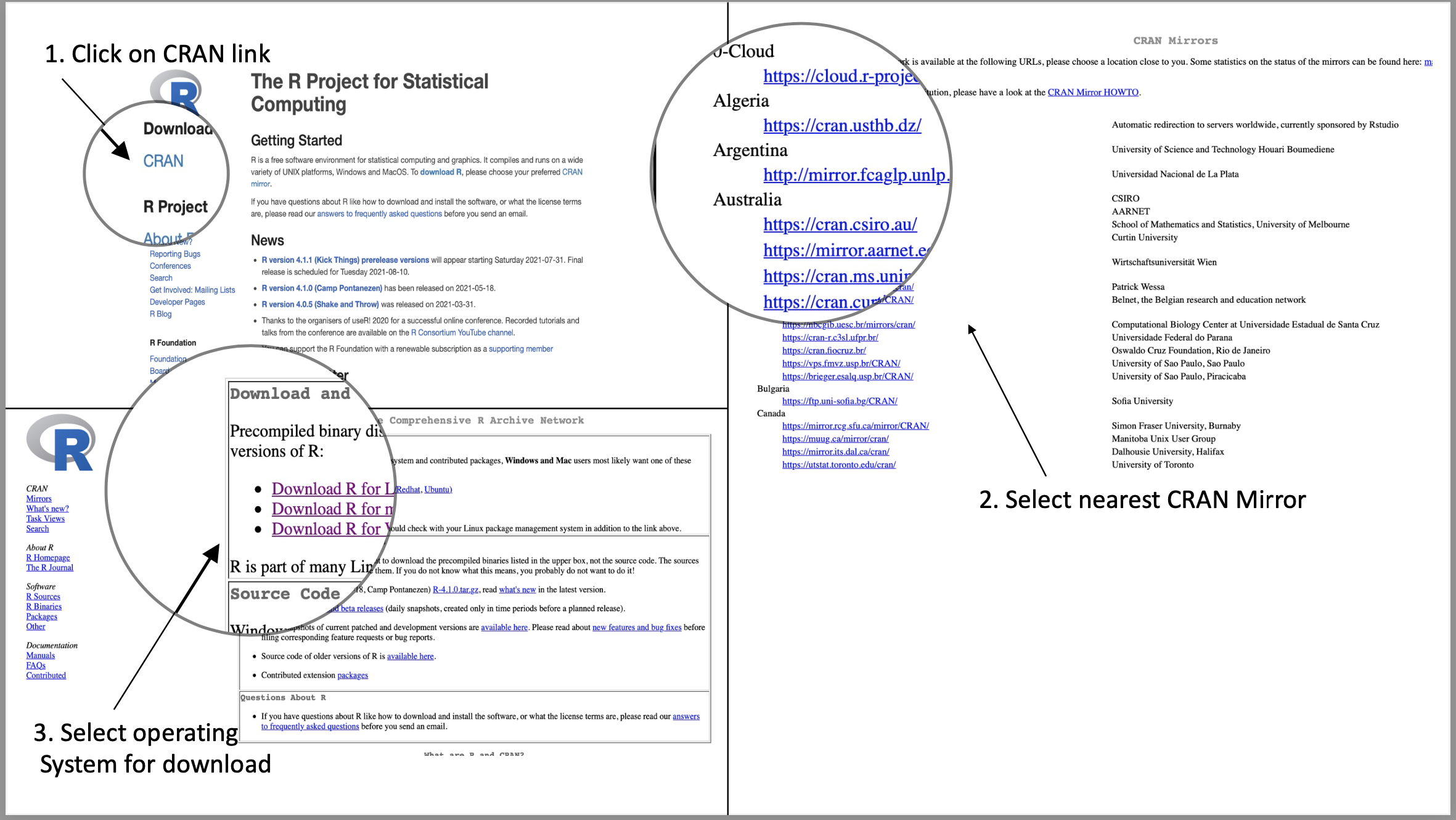
Figure 2.1: Steps in Downloading R
On each local CRAN there are separate links for the Linux, macOS, and Windows operating systems. Click on the link that matches your operating system (Step 3 in Figure 2.1). If you are using a Windows operating system, you then click on Base and you will be sent to a download link; click the download link and install the program. If you are using macOS, you will be presented with download choices based on your specific version of macOS; choose the download option whose system requirements match your operating system, and download as you would any other program from the web. For Linux, choose the distribution that matches your system and follow the installation instructions.
It is strongly recommended that you use RStudio as the working environment for running R. This is an especially important recommendation for new users. To download RStudio, go to the RStudio web page (https://www.rstudio.com/) and scroll down and click on the download button (Step 1 in Figure 2.2).5 Then, scroll down the new page, click on RStudio Desktop DOWNLOAD button, and follow instructions for downloading RStudio (Step 2 in Figure 2.2). If you have not already installed R, you can do so by clicking the link to install it (Step 3 in Figure 2.2) and go through the R installation steps described above. If you have installed R, click the DOWNLOAD RSTUDIO button to install RStudio.
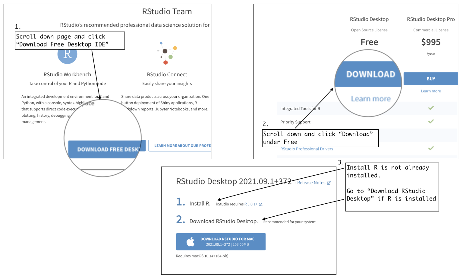
Figure 2.2: Downloading RStudio
RStudio Cloud (https://rstudio.cloud) is a terrific online alternative for doing your work in the RStudio environment without downloading R and RStudio to your personal device. This is an especially attractive alternative if your personal computer is a bit out of date or under powered. RStudio Cloud can be used by individuals for free or at a very low cost, and institutions can choose from a number of low cost options to set up free access for their students. In addition, instructors who set up a class account on RStudio Cloud can take advantage of a number of options that facilitate working with their students on assignments.
Assuming you’ve downloaded RStudio, open it by clicking on the appropriate icon or file name. When RStudio opens, it will automatically open and work with R, as long as you’ve also downloaded it. Initially, you should see three different RStudio windows that look something like the image in the first illustration below. It’s possible that your screen will look a bit different due to differences in operating systems, the version of RStudio you download, or some other reason; but, generally, it should look like Figure 2.3.
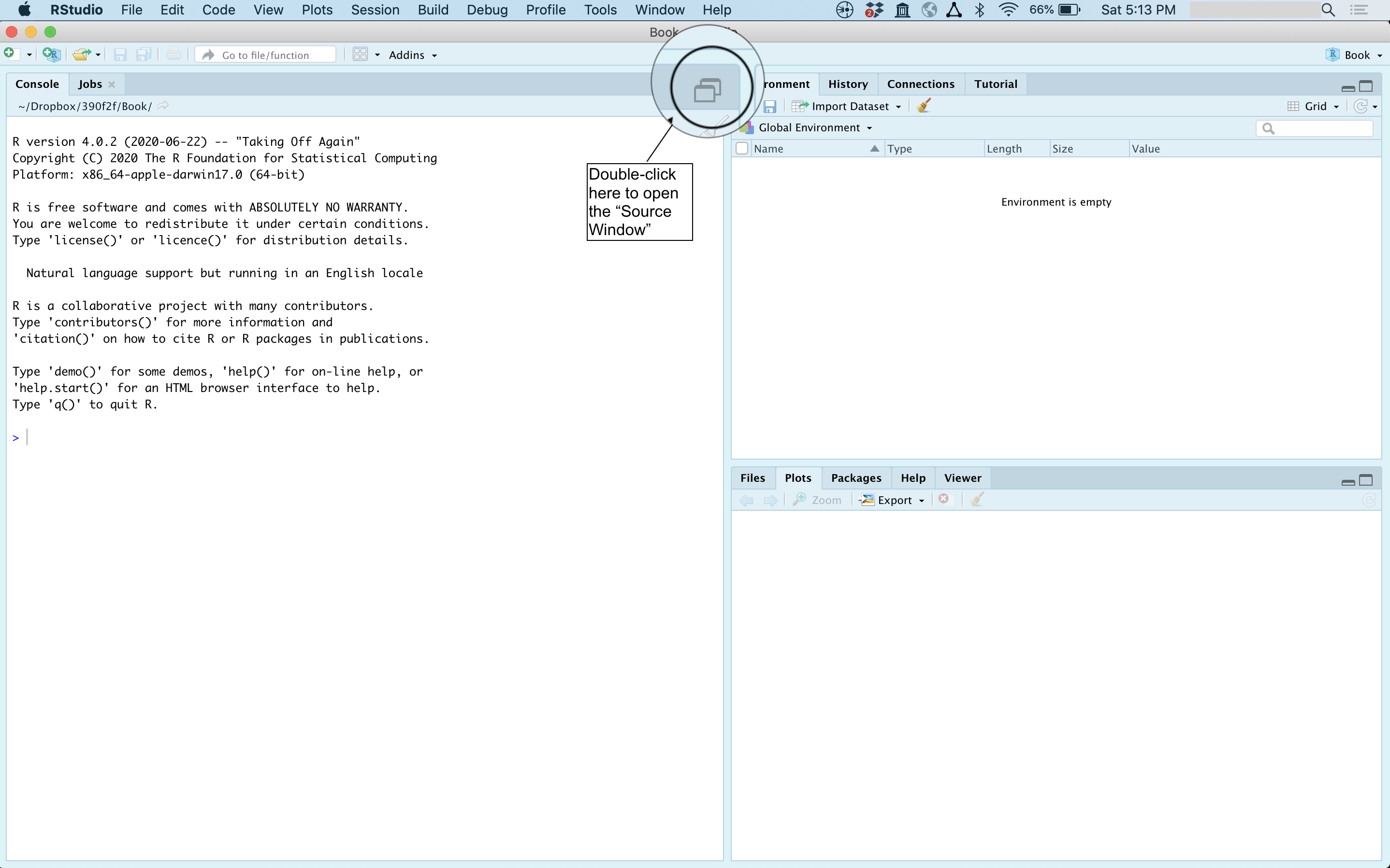
Figure 2.3: An Annoted Display of Initial RStudio Windows
The first thing you should do is click on the boxes in the upper-right corner of the Console window on the left side. This will open up an additional window, the Source window. Once you do this, your computer display should look like the image in Figure 2.4 (except for the annotations). Again, there may be some slight differences, but not enough to matter for learning about the RStudio environment.
You will use the Source window a lot. In fact, almost everything you do will originate in the Source window. There is also a lot going on in the other windows, but, generally, everything that happens (well, okay, most things) in the other windows happens because of what you do in the Source window. This is the window where you write your commands (the code that tells R what to do). Some people refer to this as the Script window because this is where you create the “script” file that contains your commands. Script files are very useful. They help you stay organized and can save you a lot of time and effort over the course of a semester or while you are working on a given research project.
Here’s how the script file works. You start by writing a command at the cursor. You then leave the cursor in the command line and click on the “Run” icon (upper-right part of the window). Alternatively, you can leave the cursor in the command line and press control(CNTRL)+return(Enter) on your keyboard. When you do this, you will see that the command is copied and processed at the > prompt in the Console window. As indicated above, what you do in the Source window controls what happens in the other windows (mostly). You control what is executed in the Console window by writing code in the Source window and telling R to run the code. You can also just write the command at the prompt in the Console window, but this tends to get messy and it is easier to write, edit, and save your commands in the Source window.
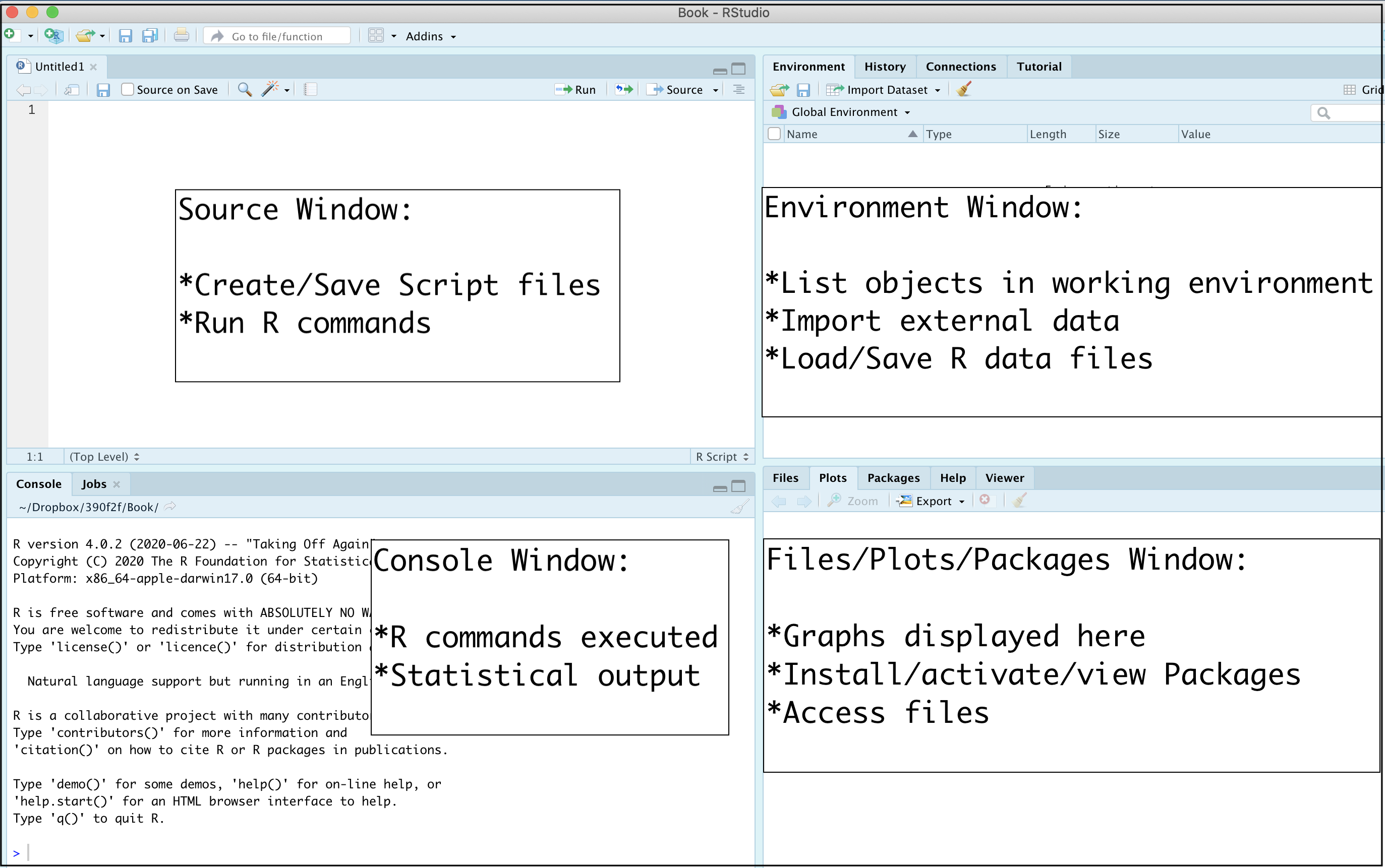
Figure 2.4: An Annotated Display of RStudio Windows
Once you execute the command, the results usually appear in one of two places, either the Console window (lower left) or the “Plots” tab in the lower right window. If you are running a statistical function, the results will appear in the Console window. If you are creating a graph, it will appear in the Plots window. If your command has an error in it, the error message will appear in the Console window. Anytime you get an error message, you should edit the command in the source window until the error is corrected, and make sure the part of the command that created the error message is deleted. Once you are finished running your commands, you can save the contents of the Source window as a script file, using the “save” icon in the upper-left corner of the window. When you want to open the script file again, you can use the open folder icon in the toolbar just above the Source window to see a list of your files. It is a good idea to give the script file a substantively meaningful name when saving it, so you know which file to access for later uses.
Creating and saving script files is one of the most important things you can do to keep your work organized. Doing so allows you to start an assignment, save your work, and come back to it some other time without having to start over. It’s also a good way to have access to any previously used commands or techniques that might be useful to you in the future. For instance, you might be working on an assignment from this book several weeks down the road and realize that you could use something from the first couple of weeks of the semester to help you with the assignment. You can then open your earlier script files to find an example of the technique you need to use. It is probably the case that most people who use R rely on this type of recovery process–trying to remember how to do something, then looking back through earlier script files to find a useful example–at least until they have acquired a high level of expertise. In fact, the writing of this textbook relied on this approach a lot!
The upper-right window in RStudio includes a number of different tabs, the most important of which for our purposes is the Environment tab, which provides a list of all objects you are using in your current session. For instance, if you import a new data set it will be listed here. Similarly, if you store the results of some analysis in a new object (this will make more sense later), that object will be listed here. There are a couple of options here that can save you from having to type in commands. First, the open-folder icon opens your working directory (the place where R saves and retrieves files) so you can quickly add any pre-existing R-formatted data sets to your environment. You can also use the Import Dataset icon to import data sets from other formats (SPSS, Stata, SAS, Excel) and convert them to data sets that can be used in R. The History tab keeps a record of all commands you have used in your R session. This is similar to what you will find in the script file you create, except that it tends to be a lot messier and includes lines of code that you don’t need to keep, such as those that contain errors, or multiple copies of commands that you end up using several times.
The lower-right window includes a lot of useful options. The Plots tab probably is the most often used tab in the lower-right window. It is where graphs appear when you run commands to create them. This tab also provides options for exporting the graphs. The Files tab includes a list of all files in your working directory. This is where your script file can be found after you’ve saved it, as well as well as any R-generated files (e.g., data sets, graphs) you’ve saved. If you click on any of the files, they will open in the appropriate window. The Packages tab lists all installed packages (bundles of functions and objects you can use–more on this later) and can be used to install new packages and activate existing packages. The Help tab is used to search for help with R commands and packages. It is worth noting that there is a lot of additional online help to be had with simple web searches. The Viewer tab is unlikely to be of much use to new R users.
This overview of the RStudio setup is only going to be most useful if you jump right in and get started. As with learning anything new, the best way to learn is to practice, make mistakes, and practice some more. There will be errors, and you can learn a lot by figuring out how to correct them.
2.2 Understanding Where R (or any program) Fits In
Before getting into the specific aspects of exactly how you tell R to do something, it is important to understand the relationship between you (the researcher), the data, and R. These connections may seem obvious to professors and experienced researchers, or to students who have had a couple of research-based courses, but they are not so obvious to a lot of students, especially those with relatively little experience. For many students, there is a black box element to the research process–they’re given some data and told what commands to use and how the results should be interpreted, but without really understanding the process that ties things together. Understanding how things fit together is important because it helps reduce user anxiety and facilitates somewhat deeper learning.
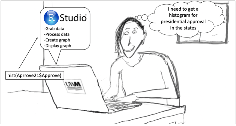
The five Panes below in the R and Amazing College Student comic strip (below) are a summary of how the researcher is connected to R and the data and how these connections produce results. The first thing to realize is that R does things (performs operations) because you tell it to. Without your ideas and input R does nothing, so you are in control. It all starts with you, the researcher. Keep this in mind as you progress through this book.
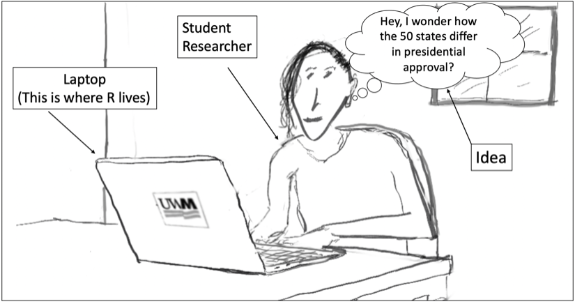
You, the college student, are sitting at your desk with your laptop, thinking about things that interest you (first pane). Maybe you have an idea about how two variables are connected to each other, or maybe you are just curious about some sort of statistical pattern. In this scenario, let’s suppose that you are interested in how the states differ from each other with respect to presidential approval in the first few months of the Biden administration. No doubt, President Biden is more popular in some states than in others, and it might be interesting to look at how states differ from each other. In actuality, you are probably interested in discovering patterns of support and testing some theory about why some states have high approval levels and some states have low approval levels. For now, though, let’s just focus on the differences in approval.
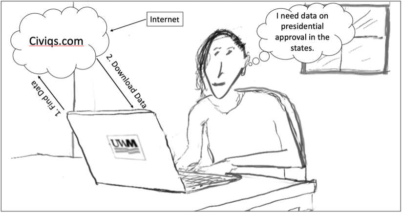
Odds are that you don’t have this information at your finger tips, so you need to go find it somewhere. You’re still sitting with your laptop, so you decide to search the internet for this information (second comic pane).
You find the data at civiqs.com, an online public opinion polling firm. After digging around a bit on the civiqs.com site, you find a page that has information that looks something like Figure 2.5.
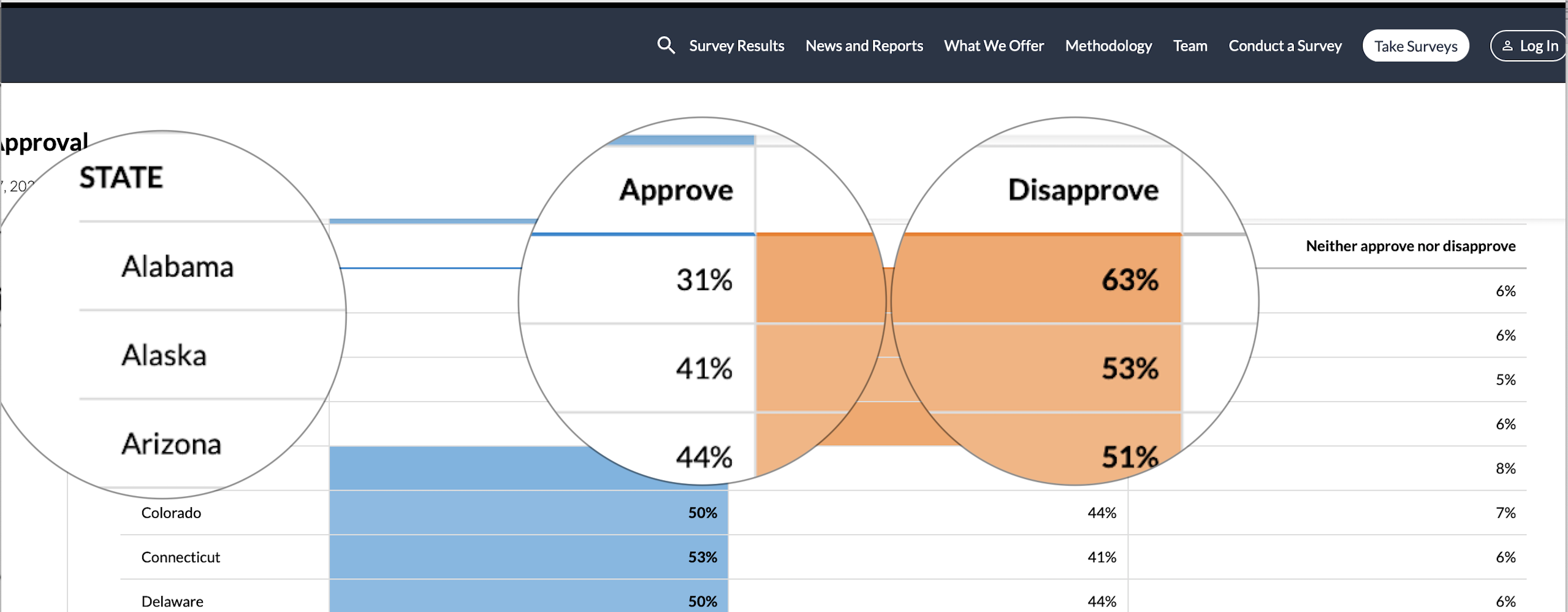
Figure 2.5: Presidential Approval data from civiqs.com
For each state, this site provides an estimate of the percent who approve, disapprove, and who neither approve nor disapprove of the way President Biden is handling his job as president, based on surveys taken from January to June of 2021. This is a really nice table but it’s still a little bit hard to make sense of the data. Suppose you want to know which states have relatively high or low levels of approval? You could hunt around through this alphabetical listing and try to keep track of the highest and lowest states, or you could use a program like R to organize and process data for you. To do this, you need to download the data to your laptop and put it into a format that R can use. (Second comic pane). In this case, that means copying the data into a spreadsheet that can be imported to R (this has been done for you), or using more advanced methods to have R go right to the website and grab the relevant data (beyond the scope of what we are doing). Once the data are downloaded, you are ready to use R.
2.3 Time to Use R
Before moving on to work with R, you need to Download the Textbook Data Sets to your computer. Go to this link (https://bit.ly/3PkyMBW), where you will find a collection of files with .rda and .xlsx extensions. Download all of these files into a directory (folder) where you want to store your work. You will be using these files throughout the remaining chapters of this book.
From this point on, the process is all about you, the researcher, requesting things from R, and R providing responses. Hopefully, R will give you what you asked for, but it might also tell you that your request created an error. That’s part of the process. The first step is to make sure the Source window in RStudio is open, so you can easily edit and save your commands from this session. If it is not open, you can reduce the size of the Console window, as instructed above, or click on the “plus” icon in the upper left corner and select “R Script.”
Now, let’s see how we can work with R to take a closer look at the presidential approval data. First things first, tell R to get the data. In RStudio, you can do this by using the Import Dataset tab in the Environment/History window. Just click on “Browse” to find the file you want to open and then click on “Import”. If you do this, the following commands will be executed (you can also just type the commands listed below into the script file and run it). Note, that you may be prompted to install a missing package (readxl), click “yes”.
#Tell R to install the `readxl` package
install.packages("readxl")
#Tell R to make "readxl" available for use
library(readxl)
#Go to the directory where you put the data, get the file, and put it in a
#new data set named "Approve21"
Approve21 <- read_xlsx("<path to data file>/Approve21.xlsx")
#See data in spreadsheet format
View(Approve21)
In highlighted segments like the one shown above, the italicized text that starts with # are comments or instructions to help you understand what’s going on, and the other lines are commands that tell R what to do. You should use this information to help you better understand how to use R
This set of commands will take the excel data file and use the read_xlsx command to convert it into a data set that R can use. Technically, this new data set is called a tibble, which is a relatively updated form of a data frame. For now, just think of this as a data set you can use in R, and we’ll get into it a bit more at the end of this chapter. The first thing you will see after importing the data is a spreadsheet view of the data set. Exit this window by clicking on the x on the right side of the spreadsheet view tab. Some of the information we get with R commands below can also be obtained by inspecting the spreadsheet view of the data set, but that option doesn’t work very well for larger data sets.
At this point, in RStudio you should see that the import commands have been executed in the Source window. Also, if you look at the Environment/History window, you should see that a data set named Approve21 has been added. This means that this data set is now available for you to use.
Usually, before jumping into producing graphs or statistics, we want to examine the data set to become more familiar with it. This is also an opportunity to make sure there are no obvious problems with the data. First, let’s check the dimensions of the data set (how many rows and columns):
[1] 50 5Ignoring “[1]”, which just tells you that this is the first line of output, the first number produced by dim() is the number of rows in the data set, and the second number is the number of columns. The number of rows is the number of cases, or observations, and the number of columns is the number of variables. According to these results, this data set had 50 cases and five variables. (if you look in the Environment/History window, you should see this same information listed with the data set as “50 obs. of 5 variables”).
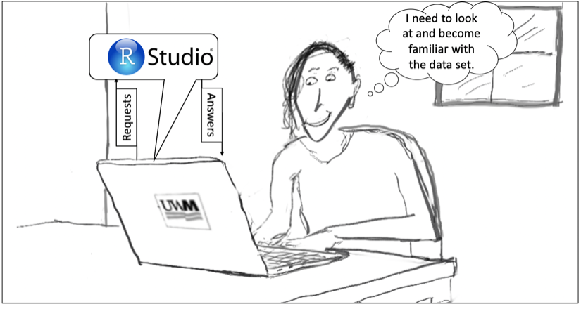
Let’s take a second to make sure you understand what’s going on here. As illustrated the comic Pane below, you sent requests to R in RStudio (“Hey R, use Approve21 as the data set, and tell me its dimensions”) and R sent information back to you. Check in with your instructor if this doesn’t make sense to you
Does 50 rows and five columns make sense, given what we know about the data? It makes sense that there are 50 rows, since we are working with data from the states, but if you look at the original data is Figure 2.5, it looks like there is an extra column. To verify that the variables and cases are what we think they are, we can tell R to show us some more information about the data set. First, we can have R show the names of the variables (columns) in the data set:
[1] "state" "stateab" "Approve" "Disapprove" "Neither" Okay, this is helpful. Now we know that the data in the first and second columns contain some sort of state identifiers, and it looks like the last three columns contain data on the percent who approve, disapprove, or neither approve or disapprove of President Biden. If you compare this to the columns in Figure 2.5, you will note that the second state identifier, stateab, was added to the data set after the data were downloaded from civiqs.com.
You can also get more information regarding the nature of the variables. Below, we use sapply() to identify the class (level of measurement) of all variables in the data set.
# sapply tells R to apply a command ("class") to all variables
# in a data set (Approve21).
sapply(Approve21, class)
state stateab Approve Disapprove Neither
"character" "character" "numeric" "numeric" "numeric" This confirms that state and stateab are character (non-numeric) variables and that the remaining variables are numeric, as expected. This is an important step because it can help flag certain types of errors. If there had been a coding error in which a stray character or symbol was entered in place of a neighboring number on the keyboard (e.g., 3o or 3p instead of 30) for Approve, then it would have shown up here as a character variable instead of the expected numeric variable.
But we don’t know from this if the data set uses a state abbreviation or the full state names to identify the cases, and we also don’t know if Approve and Disapprove are expressed as percentages or proportions. So, we need to take a closer look at the data. One useful pair of commands, head() and tail(), can be used to look at the first and last several rows in the data set.
# A tibble: 6 × 5
  state      stateab Approve Disapprove Neither
  <chr>      <chr>     <dbl>      <dbl>   <dbl>
1 Alabama    AL           31         63       6
2 Alaska     AK           41         53       6
3 Arizona    AZ           44         51       5
4 Arkansas   AR           31         63       6
5 California CA           57         35       8
6 Colorado   CO           50         44       7
Here, you see the first six rows and learn that state uses full state names, stateab is the state abbreviation, and the other variables are expressed as whole numbers. Note that this command also gives you information on the level of measurement for each variable: “chr” means the variable is a character variables, and “dbl” means that the variable is a numeric variable that could have a decimal point (though none of these variables do).
We can also look at the bottom six rows:
# A tibble: 6 × 5
  state         stateab Approve Disapprove Neither
  <chr>         <chr>     <dbl>      <dbl>   <dbl>
1 Vermont       VT           58         36       7
2 Virginia      VA           48         46       6
3 Washington    WA           53         39       7
4 West Virginia WV           23         72       5
5 Wisconsin     WI           47         48       5
6 Wyoming       WY           26         68       5
If we pay attention to the values of Approve and Disapprove in these two short lists of states, we see quite a bit of variation in the levels of support for President Biden. Not Surprisingly, the president was fairly unpopular in conservative places such as Alabama, Arkansas, West Virginia, and Wyoming, and fairly popular in more liberal states, such as California, Vermont, and Washington. However, because the data set is ordered alphabetically by state name, it is hard to get a more general sense of what types of states give President Biden high or low marks for how he is handling his job. You could “eyeball” the entire data set and try to keep track of states that are relatively high or low on presidential approval, but that is not very efficient and is probably prone to some level of error. Alternatively, you can use the head() and tail() commands but tell R to list the data set from lowest to highest approval rating rather than by state name, as it does now. We’ll do that below, but first we need to discuss how we reference specific variables when using R.
Referencing Specific Variables. In all of the commands above, we asked R to give us specific information about the data set named Approve21. Now, we want to ask R to use a specific variable from Approve21 to re-order the data. Generally, when asking R to do something with a specific variable (column) from a data set, we follow the format DatasetName$VariableName to identify the variable, separating the data set and variable name with a dollar sign. So, in order to have R sort the data by presidential approval level in the states, we identify the approval variable as Approve21$Approve. R is case sensitive, so you will get an error message if you use Approve21$approve or approve21$Approve. Make sure you understand why this is the case. (Side note: one of the nice things about using RStudio is that it auto-populates valid data set names and variable names once you’ve started typing them).
We still use the head() and tail() but add the order() command to get a listing of the lowest and highest approval states. Here, we tell R to sort the data set from lowest to highest levels of approval—Approve21[order(Approve21$Approve),]—and replace the original data set with the sorted data set.
#Sort by "Approve" and copy over original data set
Approve21<-Approve21[order(Approve21$Approve),]
#list the first several rows of data, now ordered by "Approve"
head(Approve21)
# A tibble: 6 × 5
state stateab Approve Disapprove Neither
<chr> <chr> <dbl> <dbl> <dbl>
1 West Virginia WV 23 72 5
2 Wyoming WY 26 68 5
3 Oklahoma OK 29 65 6
4 Idaho ID 30 65 5
5 Alabama AL 31 63 6
6 Arkansas AR 31 63 6This shows us the first six states in the data set, those with the lowest levels of presidential approval. Our initial impression from the alphabetical list was verified: President Biden is given his lowest marks in states that are usually considered very conservative. There is also a bit of a regional pattern, as these are all southern or mountain west states.
Now, let’s look at states with the highest approval levels by looking at the last six states in the data set. Notice that you don’t have to sort the data set again because the earlier sort changed the order of the observations until they are sorted again for some reason.
# A tibble: 6 × 5
  state         stateab Approve Disapprove Neither
  <chr>         <chr>     <dbl>      <dbl>   <dbl>
1 California    CA           57         35       8
2 Rhode Island  RI           57         37       7
3 Vermont       VT           58         36       7
4 Maryland      MD           59         33       8
5 Hawaii        HI           61         33       6
6 Massachusetts MA           63         30       7
Again, our initial impression is confirmed. President Biden gets his highest marks in states that are typically considered fairly liberal states. There is also an east coast and Pacific west flavor to this list of high approval states.
Usually, data sets have many more than five variables, so it makes sense to just show the values of variables of interest, in this case state (or stateab) and Approve, instead of the entire data set. To do this, you can modify the head and tail commands to designate that certain columns be displayed (shown below with head).
#list the first several rows of data for "state" and "Approve"
head(Approve21[c('state', 'Approve')])
# A tibble: 6 × 2
state Approve
<chr> <dbl>
1 West Virginia 23
2 Wyoming 26
3 Oklahoma 29
4 Idaho 30
5 Alabama 31
6 Arkansas 31Here, the c('state', 'Approve') portion is used to tell R to combine the columns headed by state and Approve from the data set Approve21.
If you only want to know the names of the highest and lowest states listed in order of approval, you can just use Approve21$states in the head and tail commands, again assuming the data set is ordered by levels of approval (shown below with tail).
[1] "California"    "Rhode Island"  "Vermont"       "Maryland"
[5] "Hawaii"        "Massachusetts"
The listing of states looks a bit different, but they are still listed in order, with Massachusetts giving Biden his highest approval rating.
Get a Graph. These few commands have helped you get more familiar with the shape of the data set, the nature of the variables, and the types of states at the highest and lowest end of the distribution, but it would be nice to have a more general sense of the variation in presidential approval among the states. For instance, how are states spread out between the two ends of the distribution? What about states in between the extremes listed above? You will learn about a number of statistical techniques that can give you information about the general tendency of the data, but graphing the data as a first step can also be very effective. Histograms are a particularly helpful type of graph for this purpose. To get a histogram , you need to tell R to get the data set, use a particular variable, and summarize its values in the form of a graph (as in cartoon Pane 4).
The following very simple command will produce a histogram:
#This command tells R to use the data in the "Approve" column
# of the "Approve21" data set to make a histogram.
hist(Approve21$Approve)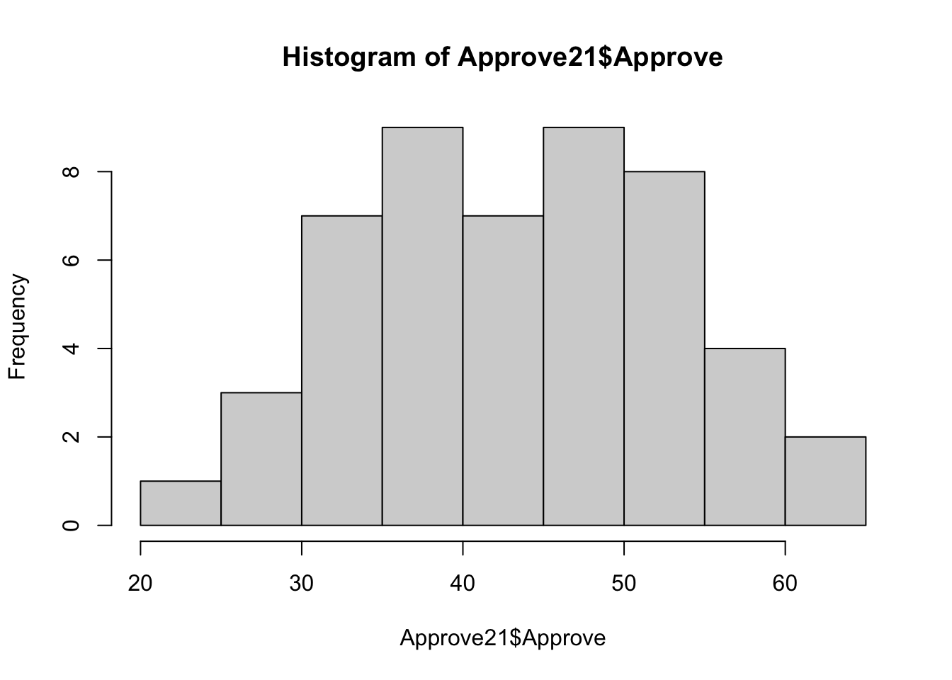
Here, the numbers on the horizontal axis represent approval levels, and the values on the vertical axis represent the number of states in each category. Each vertical bar represents a range of values on the variable of interest. You’ll learn more about histograms in the next few chapters, but you can see in this graph that there is quite a bit of variation in presidential approval, ranging from 20-25% at the low end to 60-65% at the high end (as we saw in the sorted lists), with the most common outcomes falling between 35% and 50%. So based on this graph, it looks like the distribution tilts a bit low side (less than 50% approving), but not very many states at the extremes.
One of the things you can do in R is modify the appearance of graphs to make them look a bit nicer and easier to understand. This is especially important if the information is being shared with people who are not as familiar with the data as the researcher is. In this case, you modify the graph title (main), and the horizontal (xlab) and vertical (ylab) labels:
# Axis labels in quotes and commands separated by commas
hist(Approve21$Approve,
     main="State-level Presidential Approval January-June 2021", #Graph title
     ylab="Number of States", #vertical axis label
     xlab="% Approval") #Horizontal axis label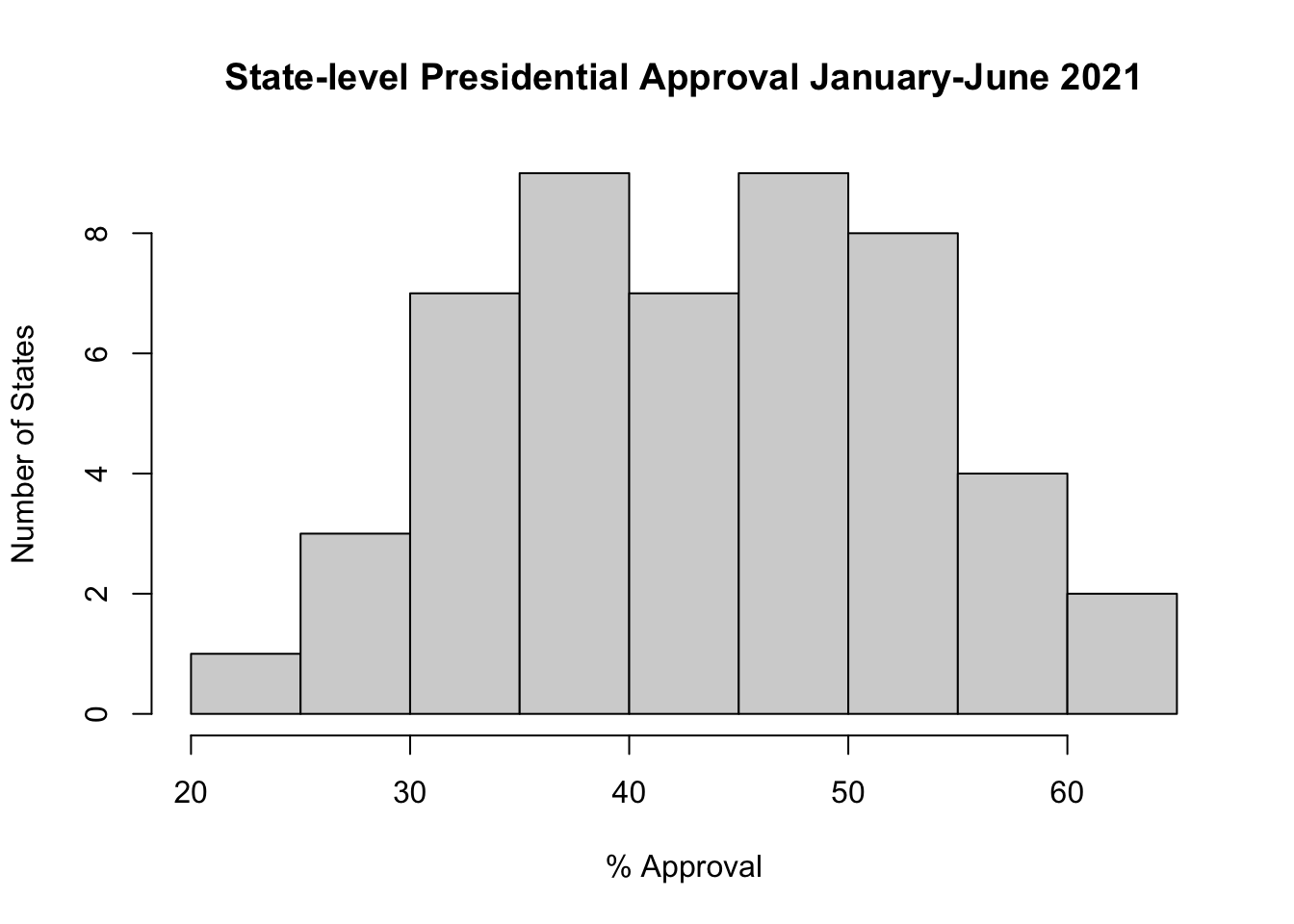
Note that all of the new labels are in quotes and the different parts of the command are separated by commas. You will get an error message if you do not use quotes and commas appropriately.
Making these slight changes to the graph improved its appearance and provided additional information to facilitate interpretation. Going back to the illustrated Panes, the cartoon student asked R for a histogram of a specific variable from a specific data set that they had previously told R to load, and R gave them this nice looking graph. That, in a nutshell is how this works. The cartoon student is happy and ready to learn more!

Before moving on, let’s check in with RStudio to see what the various windows look like after running all of the commands listed above (Figure 2.6). Here, you can see the script file (named “chpt2.R”) that includes all of the commands run above. This file is now saved in the working directory and can be used later. The Environment window lists the Approve21 data set, along with a little bit of information about it. The Console window shows the commands that were executed, along with the results for the various data tables we produced. Finally, the Plot window in the lower-right corner shows the histogram produced by the histogram command.
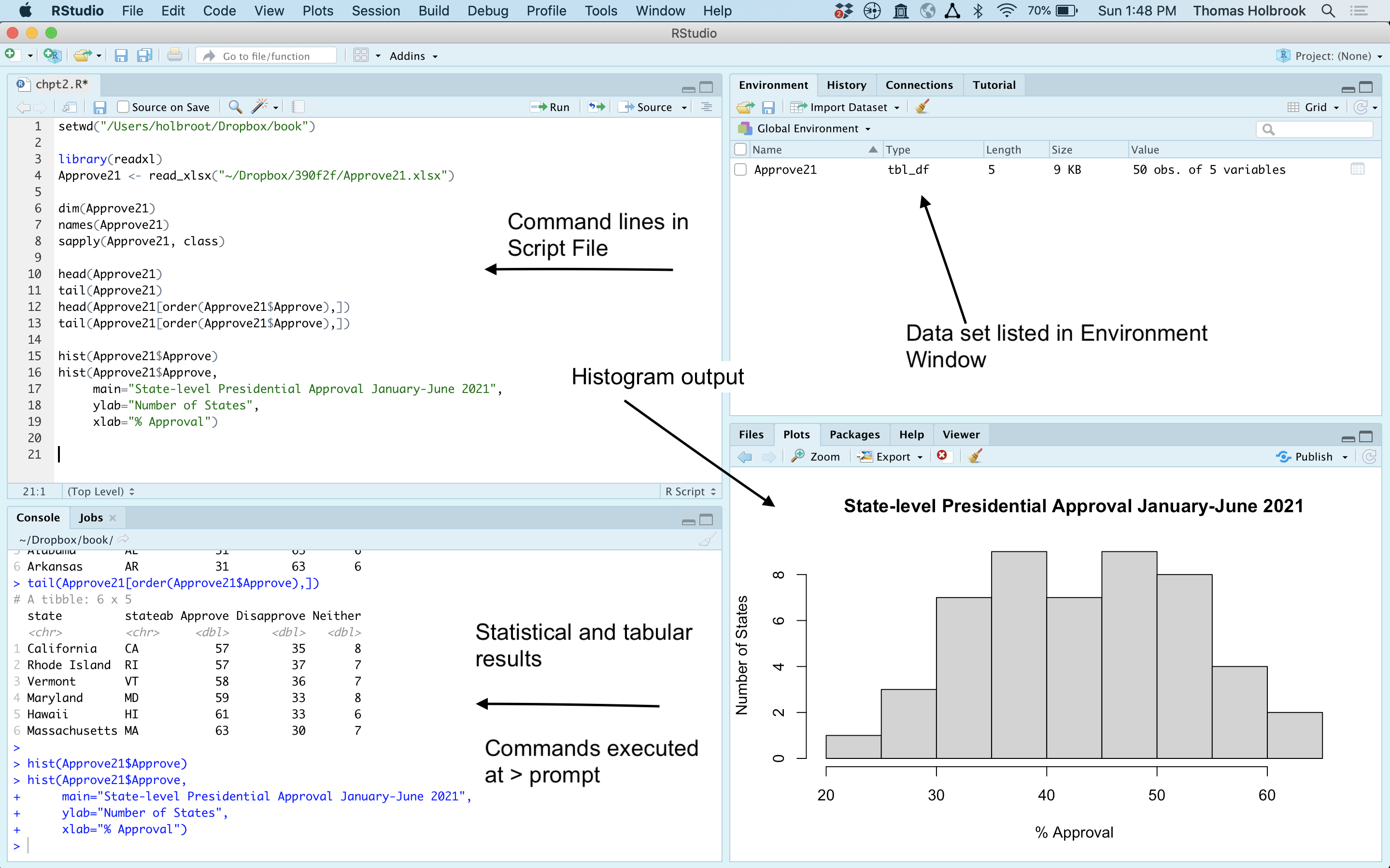
Figure 2.6: The RStudio Windows after Running Several Commands
2.4 Some R Terminology
Although it may seem a bit backward, now that you have already used R a bit, we need to cover a bit of terminology that sheds light on how R operates. It is no accident that this discussion takes place after you have already been using R. From a learning perspective, it is important to have a bit of hands-on experience with the tools you will be using before getting into definitions and terminology related to those tools. Without walking through the process of using R to produce results, much of the following discussion would be too abstract and you might have trouble making the connections between terminology and actually using R. As you will see, we have already been using many of the terms discussed below.
Data Frames. One of the most important things to understand is the concept of a data frame. A data frame is a collection of columns and rows of data, as depicted in Figure 2.7. Columns in a data frame represent the values of the variables we are interested in. The column headings are the variable names we use when telling R what to do. In Figure 2.7, the highlighted column (surrounded by a solid line) contains the state abbreviations. If you want R to use the state abbreviation, you will refer to the column as stateab. The rows represent the individual cases or observations. The highlighted row below (surrounded by the dashed line) includes information from all five columns. Although we know the second row includes outcomes for Alaska, we wouldn’t normally refer to this as “row Alaska.” Instead, from R’s perspective, this is “row 2” (the top row in a data frame is not considered row 1, as it is where the column names are stored). This collection of rows and columns together constitute a data frame (surrounded by the solid double line). For our purposes, the terms data frame and data set are used interchangeably.
One of the examples shown earlier used the names(Approve21) command get the names of all five columns (variables). In this cases, we told R to do something with the entire data set. However, when sorting the data set and also when producing the histogram, we told R to use just one column from the data set, so we specified that R should go to Approve21 and get information from the column headed by Approve, and we communicated this as Approve21$Approve.
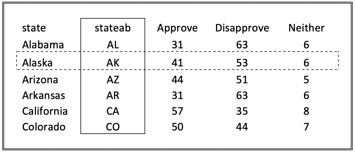
Figure 2.7: An Illustration of a Data Frame
As referenced earlier, when we imported the Approve21 data set, R created a “tibble”, which is a particular type of data set, labeled by R as tbl_df (for tibble data frame). The classic R data set is usually identified as a data.frame and has some features and characteristics that are different from a tibble data set. The default R format is data.frame but the “Import Dataset” tab in the environment creates tibbles when importing, and these tbl_df objects work better with many of the functions included in the increasingly popular tidyverse package. Both data.frame and tbl_df objects are data frames and should work equally well for all of our purposes. In instances where this is not the case, instructions will be provided to convert from one format to the other. At some level, the tibble vs. data.frame distinction is not information you need to know, so if you find this confusing, feel free to ignore it for now.
When importing and using data collected by others it can hard to connect with and understand the different elements of a data frame. One thing to do to make these things a bit more concrete is to assemble part of this data set, using the c() function in R to combine data points into vectors representing variables and then join all of those vectors using as.data.frame to create a data set. Let’s use the first four rows of data from Figure 2.7 to demonstrate this. The first variable is “state”, so we can begin by creating a vector named state that includes the first four state names in order.
#create vector of state names
state<-c("Alabama", "Alaska", "Arizona",  "Arkansas")
#Print state
state
[1] "Alabama" "Alaska" "Arizona" "Arkansas"Now, let’s do this for the first four observations of the remaining columns.
[1] 31 41 44 31[1] 63 53 51 63[1] 6 6 5 6Now, to create a data frame, we just use the data.frame function to stitch these columns together,
#Combine separate arrays into a single data frame
approval<-data.frame(state, stateab, Approve,Disapprove, Neither)
#Print the data frame
approval
state stateab Approve Disapprove Neither
1 Alabama AL 31 63 6
2 Alaska AK 41 53 6
3 Arizona AZ 44 51 5
4 Arkansas AR 31 63 6Now you have a data set with the same information found in the first few rows of data in Figure 2.7. Hopefully, this illustration helps you connect to the concept of a data frame. Fortunately, researchers don’t usually have to input data in this manner, but it is a useful tool to use occasionally to understand the concept of a data frame.
Objects and Functions When you use R, it typically is using some function to do something with some object. Everything that exists in R is an object. Usually, the objects of interest are data frames (data sets), packages, functions, or variables (objects within the data frame). We have already seen many references to objects in the preceding pages of this chapter. Many objects already exist when you download R, and many are user created. When we imported the presidential approval data, we created a new object. Even the tables we created when getting information about the data set could be thought of as objects. Functions are a particular type of objects. You can think of functions as commands that tell R what to do. Anything R does, it does with a function. Those functions tell R to do something with an object.
The code we used to create the histogram also includes both a function and an object:
hist(Approve21$Approve, main="State-level Presidential Approval 2017-19",
     xlab="% Approval", col="gray")
In this example, hist is a function call (telling R to use a function called “hist”) and Approve21$Approve is an object. The function hist is performing operations on the object Approve21$Approve. Other “action” parts of the function are main, xlab, and ylab, which are used to create the main title, and the labels for the x axis, and the y axis. Finally, the graph created by this command is a new object that appears in the “Plots” window in RStudio.
We also just used two functions (c and as.data.frame) to create six objects: the five vectors of data (state, stateab, Approve, Disapprove, and Neither) and the data frame where they were joined (approval).
Here are a few other examples of functions and objects we have used in this chapter:
| Command | Function | Object |
|---|---|---|
| read_xlsx(“Approve21.xlsx”) | read_xlsx | Approve21.xlsx |
| dim(Approve21) | dim() | Approve21 |
| head(Approve21) | head() | Approve21 |
| tail(Approve21) | tail() | Approve21 |
| sapply(Approve21, class) | sapply(), class() | Approve21 |
Storing Results in New Objects One of the really useful things you can do in R is create new objects, either to store the results of some operation or to add new information to existing data sets. For instance, at the very beginning of the data example in this chapter, we imported data from an Excel file and stored it in a new object named Approve21. This new object was used in all of the remaining analyses. You will see objects used a lot for this purpose in the upcoming chapters. We also updated an object when we sorted Approve21 and replaced the original data with sorted data. We can also modify existing data sets by creating new variables based on transformations of existing variables (more on this in Chapter 4). For instance, suppose that you want to express presidential approval as a proportion instead of a percent. You can do that by dividing Approve21$Approve by 100, but we don’t want to replace the original variable, so you store the results in a new variable, Approve21$Approve_prop, that is added to the original data set.
You might have noticed that I used <- to tell R to put the results of the calculation into a new object (variable). Pay close attention to this, as you will use the <- a lot. This is a convention in R that I think is helpful because it is literally pointing at the new object and saying to take the result of the right side action and put it in the object on the left. That said, you could write this using = instead of <- (Approve21$Approve_prop=Approve21$Approve/100) and you would get the same result. I favor using <- rather than =, but you should use what you are most comfortable with.
You can check with the names function to see if the new variable is now part of the data set.
[1] "state"        "stateab"      "Approve"      "Disapprove"   "Neither"
[6] "Approve_prop"
We see it listed as the sixth variable in the data set. you can also look at its values to make sure they are expressed as proportions rather than percentages. Typing just object name at the > prompt will generate a listing of all values for that object:
 [1] 0.23 0.26 0.29 0.30 0.31 0.31 0.31 0.32 0.33 0.34 0.35 0.36 0.36 0.36 0.37
[16] 0.37 0.37 0.39 0.39 0.39 0.41 0.41 0.42 0.43 0.44 0.44 0.45 0.46 0.47 0.47
[31] 0.47 0.48 0.48 0.50 0.50 0.50 0.51 0.52 0.52 0.52 0.53 0.53 0.53 0.54 0.57
[46] 0.57 0.58 0.59 0.61 0.63
It looks like all of the values of Approve21$Approve_prop are indeed expressed as proportions. One quick but important reminder of something mentioned earlier is in order when reading this type of output. The bracketed numbers do not represent values of the object. Instead, they tell the order of the outcomes in the data set. For instance [1] is followed by .23, .26, and 29, indicating the value of the first observation is .23, the second is .26, and the third is .29. Likewise, [16] is followed by .37, .37, and .39, indicating the value for the sixteenth observation is .37, the seventeenth is .37, and the eighteenth is .39, and so on.
Packages and Libraries A couple of other terms you should understand are package and library. Packages are collections of functions, objects (usually data sources), and code that enhance the base functions of R. For instance, the function hist() is part of a package called graphics that is automatically installed as part of the R base. And the function read_xlsx is part of a package called readxl. Once you have installed a package, you should not have to reinstall it unless you start an R session on a different device.
If you need to use a function from a package that is not already installed, you use the following command:
You can also install packages using the “Packages” tab in the lower right window in RStudio. Just go to the “Install” icon, search for the package name, and click on “Install”. When you install a package, you will see a lot of stuff happening in the Console window. Once the > prompt returns without any error messages, the new package is installed. In addition to the core set of packages that most people use, we will rely on a number of other packages in this book.
Each chapter will begin with a list of the packages that will be used, and you can install them the, if you wish. Alternatively, you can copy, paste, and run the code below to install all of the packages used in this book in one fell swoop
install.packages(c("dplyr","desc","DescTools","effectsize","gplots",
                   "Hmisc","lmtest","plotrix","ppcor","readxl","sandwich",
                   "stargazer"))
If your instructor is using RStudio Cloud, one of the benefits of that platform is that they can pre-load the packages, saving students the sometimes frustrating process of installing packages.
Libraries are where the packages are stored for active use. Even if you have installed all of the required packages, you generally can’t use them unless you have loaded the appropriate library. All chapters begin with a list of libraries you need to load.
You can also load a library by going to the “Packages” tab in the lower-right window and clicking on the box next to the already installed package. This command makes the package available for you to use. For instance, I used the command library(readxl) before using read_xlsx() to import the presidential approval data. Doing this told R to make the functions in readxl available for me to use. If I had not done this, I would have gotten an error message something like “Error: could not find function read_xlsx.” You will also get this error if you misspell the function name (happens a lot). Installing the packages and attaching the libraries allows us to access and use any functions or objects included in these packages.
Working Directory When you create files, ask R to use files, or import files to use in R, they are stored in your working directory. Organizationally, it is important to know where this working directory is, or to change its location so you can find your work when you want to pick it up again. By default, the directory where you installed RStudio is designated the working directory. In R, you can check on the location of the working directory with the getwd() command. I get something like the following when I use this command:
[1] “/Users/username/Dropbox/foldername”
In this case, the working directory is in a Dropbox folder that I use for putting together this book (I modified the path here to keep it simple). If I wanted to change this to something more meaningful and easier to remember, I could use the setwd() function. For instance, as a student, you might find it useful to create a special folder on you desktop for each class.
# Here, the working directory is set to a folder on my desktop,
# named for the data analysis course I teach.
setwd("/Users/username/Desktop/PolSci390")
I’m fine with the current location of the working directory, so I won’t change it, but you should make sure that yours is set appropriately. The nice thing about keeping all of your work (data files, script files, etc.) in the working directory is that you do not have to include the sometimes cumbersome file path names when accessing the files. So, instead of having to write something like readxl("/Users/username/Desktop/PolSci390/Approve21.xlsx"), you just have to write readxl("Approve21.xlsx"). If you need to use files that are not stored your working directory and you don’t remember their location, you can use the file.choose() command to locate them on your computer. The output from this command will be the correct path and file name, which you can then copy and paste into R.
2.4.1 Save Your Work
Before wrapping up the material in this chapter, you should save your work. This means not just saving the script file, but also saving the Approve21 data set as an R data file. To save the script file, just go to the file icon at the top of the Source Window, click the icon, and assign your file a name that is connected to the work you’ve done here and that you will be able to remember. I use “chpt2” as the name, which R saves as chpt2.R. Now, any time you need to use commands from this, you can click on the folder icon at the top of the RStudio window, locate the file, and open it.
you can also save the Approve21 data set as an R data file so you won’t need to import the Excel version of this data set when you want to use it again. The command for saving an object as an R data file is save(objectname, file=filename.rda). Here, the object is Approve21 and I want to keep that name as the file name, so I use the following command:
This will save the file to your working directory. If you want to save it to another directory, you need to add the file path, something like this:
Now, when you want to use this file in the future, you can use the load() command to access the data set.
Copy and Paste Results Finally, when you are doing R homework, you generally should show all of the final results you get, including the R code you used, unless instructed to do otherwise. This means you need to copy and past the findings into another document, probably using Microsoft Word or some similar product. When you do this, you should make sure you format the pasted output using a fixed-width font (“Courier”, “Courier New”, and “Monaco” work well). Otherwise, the columns in the R output will wander all over the place, and it will be hard to evaluate your work. You should always check to make sure the columns are lining up on paper the same way they did on screen. You might also have to adjust the font size to accomplish this.
To copy graphs, you can click “Export” in the graph window and save your graph as an image (make sure you keep track of the file location). Then, you can insert the graph into your homework document. Alternatively, you can also click “copy to clipboard” after clicking on “Export” and copy and paste the graph directly into your document. You might have to resize the graphs after importing, following the conventions used by your document program.
You may have to deal with other formatting issues, depending you what document software you are using. The main thing is to always take time to make sure your results are presented as neatly as possible. Also, it is usually best to include only your final results, unless instructed otherwise. There usually is no need to include all of the iterations you went through to get the final results. Doing so can make for sloppy and difficult-to-read homework. You should include error messages only if you were unable to get something to work and you want to receive feedback and perhaps some credit for your efforts.
2.5 Next Steps
Everything in this chapter will help you get started on your journey to using R for Political and Social Data Analysis. That said, this information is really just the very small piece of the tip of a very large iceberg of information. There is a lot more to learn. I say this not to intimidate or cause concern, but because I think this is reason for excitement. For most students, doing data analysis and working with R are both new experiences, and that’s exactly what makes this an exciting opportunity. This book is designed to make it possible for any student to learn and improve their skill level, as long as they are willing to commit to putting in the time and effort required.
You will learn more about data analysis and additional R commands in the next several chapters, and you probably will suffer through some frustration as R spits out the occasional error messages, but if you stay on top of things (on schedule, or ahead of schedule) and ask for help before its too late, you should be fine.
2.6 Exercises
2.6.1 R Problems
I tried to load the
anes20.rdadata file using the following command:load(Anes20.rda). It didn’t work. I got the following message. Error in load(Anes20.rda) : object ‘Anes20.rda’ not found I can’t figure this out. What did I do wrong?Load the
countries2data set and get the names of all of the variables included in it. Based just on what you can tell from the variable names, what sorts of variables are in this data set? Identify one variable that looks like it might represent something interesting to study (a potential dependent variable), and then identify another variable that you think might be related to the first variable you chose.Use the
dimfunction to tell how many variables and how many countries are in the data set.Use the
Approve21data set and create a new object,Approve21$net_approve, which is calculated as the percent in the state who approve of the Biden’s performance MINUS the percent in the state who disapprove of Biden’s performance. Sort the data set by `Approve21$net_approveand list the six highest and lowest states. Say a few words about the types of states in these two lists. Finally, produce a histogram ofApprove21$net_approveand describe what you see. Provide substantively meaningful labels for the histogram.
As RStudio grows in use, this web pages also changes a bit so you might find that things don’t always look the way they are presented here.↩︎