Chapter 17 Advanced Regression Topics
17.1 Get Started
In this chapter, we take up the analysis of life expectancy by taking into account other factors that might be related to health conditions in general. We will also address a few important issues related to evaluating multiple regression models. If you want to follow along in R, you should load the countries2 data set, as well as the libraries for the DescTools and stargazer packages.
17.2 Incorporating Access to Health Care
One set of variables that we haven’t considered but that should be related to life expectancy are factors that measure access to health care. Generally speaking, countries with greater availability of health care resources (doctor, hospitals, research centers, etc) should have higher levels of life expectancy. In the table below, we expand the regression model to include two additional variables, percent of the population living in urban areas and the number of doctors per 10,000 persons. Both of these variables are expected to be positively related to life expectancy, as they are linked to the availability of health care services and facilities. Doctors per 10,000 persons is a direct measure of access to health care (literally, more widely available health care), and levels of access to health care are generally lower in rural areas than in urban areas.
These variables are added in the model below:
#Add % urban and doctors per 10k to the model
fit<-lm(countries2$lifexp~countries2$fert1520 +
          countries2$mnschool+ log10(countries2$pop19_M)+
          countries2$urban+countries2$docs10k)
#Use information in 'fit' to create table of results
stargazer(fit, type="text",
          dep.var.labels=c("Life Expectancy"), #Dependent variable label
          covariate.labels = c("Fertility Rate", #Indep Variable Labels
                               "Mean Years of Education",
                               "Log10 Population", "% Urban",
                               "Doctors per 10,000"))
===================================================
                            Dependent variable:
                        ---------------------------
                              Life Expectancy
---------------------------------------------------
Fertility Rate                   -3.237***
                                  (0.341)

Mean Years of Education           0.413**
                                  (0.163)

Log10 Population                   0.082
                                  (0.331)

% Urban                          0.050***
                                  (0.015)

Doctors per 10,000                0.049*
                                  (0.027)

Constant                         73.923***
                                  (2.069)

---------------------------------------------------
Observations                        179
R2                                 0.768
Adjusted R2                        0.761
Residual Std. Error          3.606 (df = 173)
F Statistic              114.590*** (df = 5; 173)
===================================================
Note:                   *p<0.1; **p<0.05; ***p<0.01
Here’s how I would interpret the results:
The first thing to note is that four of the five variables are statistically significant (counting
docs10kas significant with a one-tailed test), and the overall model fit is improved. The only variable that has no discernible impact is population size. The model R2 is now .768, indicating that the model explains 76.8% of the variation in life expectancy, and the adjusted R2 is .735, an improvement over the previous three-variable model (adjusted R2 was .721). Additionally, the RMSE is now 3.606, also signaling less error compared to the previous model (3.768). Interpretation of the individual variables should be something like the following:Fertility rate is negatively and significantly related to life expectancy. For every one unit increase in the value of fertility rate, life expectancy is expected to decline by about 3.24 years, controlling for the influence of the other variables in the model.
Average years of education is positively related to life expectancy. For every unit increase in education level, life expectancy is expected to increase by about .413 years, controlling for the influence of the other variables in the model.
Percent urban population is positively related to life expectancy. For every unit increase in the percent of the population living in urban areas, life expectancy is expected to increase by .05 years, controlling for the influence of other variables in the model.
Doctors per 10,000 population is positively related to life expectancy. For every unit increase in doctors per 10,000 population, life expectancy is expected to increase by about .05 years, controlling for the influence of the other variables in the model.
I am treating the docs10k coefficient as statistically significant even though the p-value is greater than .05. This is because the reported p-value (< .10) is a two-tailed p-value, and if we apply a one-tailed test (which makes sense in this case), the p-value is cut in half and is less than .05. In this case, the two-tailed p-value (not shown in the table) is .068, so the one-tailed value is .034. Still, in a case like this, where the level of significance if borderline, it is best to assume that the effect is pretty small. A weak effect like this is kind of surprising for this variable, especially since there are strong substantive reasons to expect greater access to health care to be strongly related to life expectancy. Can you think of an explanation for this? We explore a couple of potential explanations for this weaker-than-expected relationship in the next two sections.
One final thing that you need to pay attention to in this model, or whenever you work with multiple regression, or any other statistical technique that involves working with multiple variables at the same time, is the number of missing cases. Missing cases occur on a given variable when cases do not have any valid outcomes. We discussed this a bit earlier in the book in the context of public opinion surveys, where missing data usually occur because people refuse to answer questions or do not have an opinion to offer. When working with aggregate cross-national data, as we are here, missing outcomes usually occur because the data are not available for some countries on some variables. For instance, some countries may not report data on some variables to the international organizations (e.g., World Bank, United Nations, etc.) that are collecting data, or perhaps the data gathering organizations collect certain types of data from certain types of countries but not for others. This is a more serious problem for multiple regression than simple regression because multiple regression uses “listwise” deletion of missing data, meaning that if a case is missing on one variable it is dropped from all variables. This is why it is important to pay attention to missing data as you add more variables to the model. It is possible that one or two variables have a lot of missing data, and you could end up making generalizations based on a lot fewer data points than you realize. At this point, using this set of five variables there are sixteen missing cases (there are 195 countries in the data set and 179 observations used in the model).47 This is not too extreme but is something that should be monitored.
17.3 Multicollinearity
One potential explanation for the tepid role of docs10k in the life expectancy model is multicollinearity. Recall from the discussions in Chapters 14 and 16 that when independent variables are strongly correlated with each other, the simple bi-variate relationships are usually overstated and the independent variables lose strength when considered in conjunction with other overlapping explanations. Normally, this is not a problem. In fact, one of the virtues of regression analysis is that the model sorts out overlapping explanations (this is why we use multiple regression). However, when the degree of overlap is too high, it can make it difficult for substantively important variables to demonstrate statistical significance. Perfect collinearity violates a regression assumption (see next chapter), but high level of collinearity can also cause problems, especially for interpreting significance levels.
Here’s how this problem comes about: the t-score for a regression coefficient (\(b\)) is calculated as \(t=\frac{b}{S_b}\), and the standard error of b (\(S_b\)) for any given variable is directly influenced by how that variable is correlated with other independent variables. The formula below illustrates how collinearity can affect the standard error of \(b_1\) in a model with two independent variables:
\[S_{b_1}=\sqrt{\frac{RMSE}{\sum(x_i-\bar{x}_1)^2(1-R^2_{1\cdot2})}}\]
As the correlation (and R2) between x1 and x2 increases, the \(S_{b_1}\) (the denominator) increases, and the t-score decreases. Because of this, high correlations among independent variables can make it difficult for variables to become statistically significant. This problem can be compounded when there are multiple strongly related independent variables This problem is usually referred to as high multicollinearity, or high collinearity.
When you have good reasons to expect a variable to be strongly related to the dependent variable and it is not statistically significant in a multiple regression model, you should think about whether collinearity could be a problem. So, is this a potential explanation for the borderline statistical significance for docs10k? It does make sense that docs10k is strongly related to other independent variables, especially since most of the variables reflect an underlying level of economic development. As a first step toward diagnosing this, let’s look at the correlation matrix for evidence of collinearity:
#Create "logpop" variable for exporting
countries2$logpop<-log10(countries2$pop19_M)
#Copy DV and IVs to new data set.
lifexp_corr<-countries2[,c("lifexp", "fert1520", "mnschool",
                           "logpop", "urban", "docs10k")]
#Restrict digits in output to fit columns together
options(digits = 3)
#Use variable in 'life_corr' to produce correlation matrix
cor(lifexp_corr, use = "complete") #"complete" drops missing data
lifexp fert1520 mnschool logpop urban docs10k
lifexp 1.0000 -0.8399 0.7684 -0.0363 0.6024 0.7031
fert1520 -0.8399 1.0000 -0.7627 0.0706 -0.5185 -0.6777
mnschool 0.7684 -0.7627 1.0000 -0.0958 0.5787 0.7666
logpop -0.0363 0.0706 -0.0958 1.0000 0.0791 -0.0168
urban 0.6024 -0.5185 0.5787 0.0791 1.0000 0.5543
docs10k 0.7031 -0.6777 0.7666 -0.0168 0.5543 1.0000Look across the row headed by docs10k, or down the docs10k column to see how strongly it is related the the other variables. First, there is a strong bivariate correlation (r=.70) between doctors per 10,000 population and the dependent variable, life expectancy. Further, docs10k is also highly correlated with fertility rates (r= -.68), mean years of education (r=.77), and percent living in urban areas (r= .55). Based on these correlations, it seems plausible that collinearity could be causing a problem for the significance of slope for docs10k.
There are two important statistics that help us evaluate the extent of the problem with collinearity: The tolerance and VIF (variance inflation) statistic. Tolerance is calculated as:
\[ \text{Tolerance}_{x_1}=1-R^2_{x_1,x_2\cdot \cdot x_k}\]
You should recognize this from the denominator of the formula for the standard error of the regression slope; it is the part of the formula that inflates the standard error. Note that as the percent of variation in x1 that is accounted for by the other independent variables increases, the tolerance value decreases. The tolerance is the proportion of variance in an independent variable that is not explained by variation in the other independent variables.
The VIF statistic tells us how much the variance in the slope is inflated due to inter-item correlation. The calculation of the VIF is based on the tolerance statistic:
\[\text{VIF}_{b_1}=\frac{1}{\text{Tolerance}_{b_1}}\]
We can calculate tolerance for docs10k stats by regressing it on the other independent variables to get \(R^2_{x_1,x_2\cdot \cdot x_k}\) . In other words, treat docs10k as a dependent variable and see how much of its variation is accounted for by the other variables in the model. The model below does this:
#Use 'docs10k' as the DV to Calculate its Tolerance
fit_tol<-lm(countries2$docs10k~countries2$fert1520 + countries2$mnschool
            + log10(countries2$pop19_M) +countries2$urban)
#Use information in 'fit_tol' to create a table of results
stargazer(fit_tol, type="text",
          title="Treating 'docs10k' as the DV to Calculate its Tolerance",
          dep.var.labels=c("Doctors per 10,000"),
          covariate.labels = c("Fertility Rate",
                               "Mean Years of Education",
                               "Log10 Population", "% Urban"))
Treating 'docs10k' as the DV to Calculate its Tolerance
===================================================
                            Dependent variable:
                        ---------------------------
                            Doctors per 10,000
---------------------------------------------------
Fertility Rate                   -2.560***
                                  (0.947)

Mean Years of Education          2.860***
                                  (0.406)

Log10 Population                   0.754
                                  (0.934)

% Urban                           0.099**
                                  (0.043)

Constant                          -6.080
                                  (5.840)

---------------------------------------------------
Observations                        179
R2                                 0.623
Adjusted R2                        0.615
Residual Std. Error          10.200 (df = 174)
F Statistic               71.900*** (df = 4; 174)
===================================================
Note:                   *p<0.1; **p<0.05; ***p<0.01
Note that the R2=.623, so 62.3 percent of the variation in docs10k is accounted for by the other independent variables. Using this information, we get:
Tolerance: 1-.623 = .377.
VIF (1/tolerance): 1/.377 = 2.65
So, is a VIF of 2.65 a lot? In my experience, no, but it is best to evaluate this number in the context of the VIF statistics for all variables in the model. Instead of calculating all of these ourselves, we can just have R get the VIF statistics for us:
      countries2$fert1520       countries2$mnschool log10(countries2$pop19_M)
                     2.55                      3.50                      1.04
         countries2$urban        countries2$docs10k
                     1.63                      2.65
Does collinearity explain the marginally significant slope for docs10k? Yes and no. Sure, the slope for docs10k would probably have a smaller p-value if we excluded the variables that are highly correlated with it, but some loss of impact is almost always going to happen when using multiple regression; that’s the point of using it! Also, the issue of collinearity is not appreciably worse for docs10k than it is for fertility rate, and it is less severe that it is for mean education, so it’s not like this variable faces a higher hurdle than the others. Based on these results I would conclude that collinearity is a slight problem for docs10k, but that there is probably a better explanation for its level of statistical significance. There is no magic cutoff point for determining that collinearity is a problem that needs to be addressed. In my experience, VIF values less than 10 are probably not worth worrying about, but that is a judgment call and you always have to consider issues like this in the context of the data and model you are using.
Even though collinearity is not a big problem here, it is important to consider what to do if there is extreme collinearity a regression model. Some people suggest dropping a variable, possibly the one with the highest VIF. I don’t generally like to do this, but it is something to consider, especially if you have several variables that are measuring different aspects of the same concept and dropping one of them would not hurt your ability to measure an important concept. For instance, suppose this model also included hospital beds per capita and nurses per capita. These variables, along with docs10k all measure different aspects of access to health care and should be strongly related to each other. If there were high VIF values for these variables, we could probably drop one or two of them to decrease collinearity, and we would still be able to consider access to health care as an explanation of differences in life expectancy.
Another alternative that would work well in this scenario would be to combine the highly correlated variables into an index that uses information from all of the variables to measure wealth with a single index. We did something like this in Chapter 3 where we created a single index of LGBTQ policy preferences based on outcomes from several separate LGBTQ policy questions. Indexing like this minimizes the collinearity problem without dropping any variables. There are many different ways to combine variables, but expanding on that here is a bit beyond the scope of this book.
17.4 Checking on Linearity
The relationship between docs10k and life expectancy presents an opportunity to explore another important potential problem that can come up in regression analysis. Theoretically, there should be a relatively strong relationship between these two variables, not one whose statistical significance in the multiple regression model depends upon whether you are using one- or two-tailed test. We have already explored collinearity as an explanation for the weak showing of docs10k, but that does not appear to be the primary explanation. While the bivariate correlation (r=.70) is reported above, one thing we did not do earlier was examine a simple scatterplot for this relationship. Let’s do that now to see if it offers any clues.
#Scatterplot of "lifexp" by "docs10k"
plot(countries2$docs10k, countries2$lifexp, ylab="Life Expectancy",
     xlab="Doctors per 10k Population")
#Add linear regression line
abline(lm(countries2$lifexp~countries2$docs10k))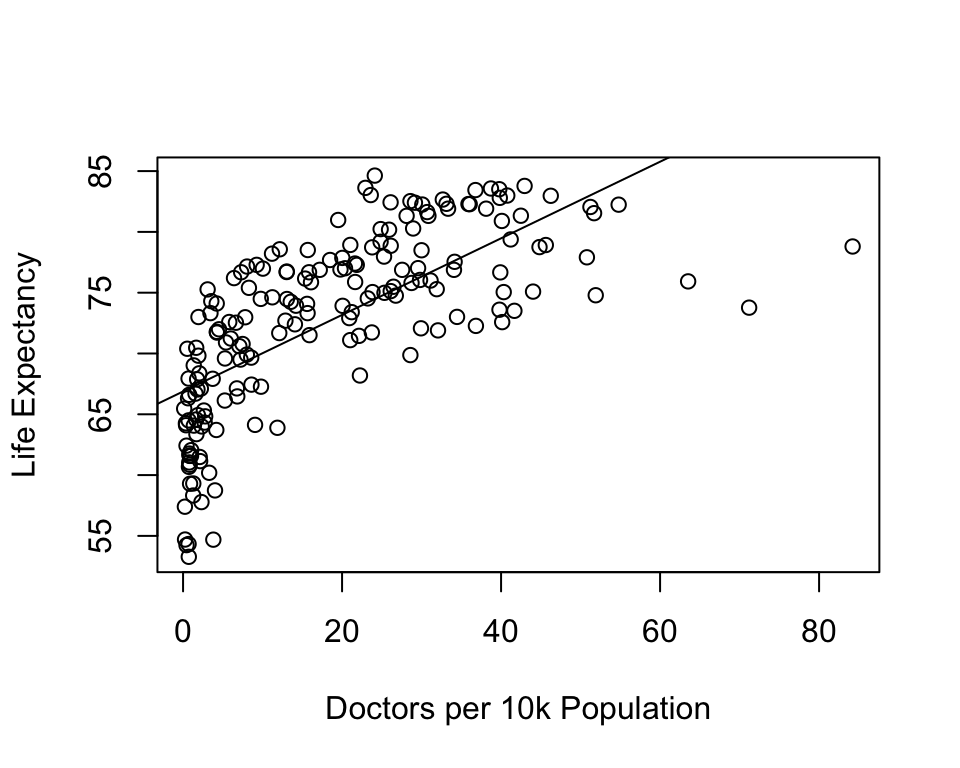
This is interesting. Note that the linear prediction line does not seem to fit the data in the same way we have seen in most of the other scatterplots. Focusing on the pattern in the markers, this doesn’t look like a typical linear pattern. At low levels of the independent variable there is a lot of variation in life expectancy, but, on average, it is fairly low. Increases in doctors per 10k from the lowest values to 14 or so leads to substantial increases in life expectancy but then there are diminishing returns from that point on. Looking at this plot, you can imagine that a curved line would fit the data points better than the existing straight line. One of the important assumptions of OLS regression is that all relationships are linear, that the expected change in the dependent variable for a unit change in the independent variable is constant across values of the independent variables. This is clearly not the case here. Sure, you can fit a straight line to the pattern in the data, but if the pattern in the data is not linear, then the line does not fit the data as well as it could, and we are violating an important assumption of OLS regression (see next Chapter).
There are a couple of ways to model non-linear relationships in regression analysis. Just as \(y=a + bx\) is the equation for a straight line, there are a number of possibilities for modeling a curved line. Based on the pattern in the scatterplot–one with diminishing returns–I would opt for the following model:
\[\hat{y}=a + b*log_{10}x\]
Here, we transform the independent variable by taking the logged values of its outcomes.
Log transformations are very common, especially when data show a curvilinear pattern or when a variable is heavily skewed. In this case, we are using a log(10) transformation. This means that all of the original values are transformed into their logged values, using a base of 10. A logged value is nothing more than the power to which you have to raise your log base (in this case, 10) in order to get the original raw score. For instance, log10 of 100 is 2, because 102=100, and log10 of 50 is 1.699 because 101.699=50, and so on. We have used log10 for population size since Chapter 14, and you may recall that a logged version population density was used in one of the end-of-chapter assignments in Chapter 16. Using logged values has two primary benefits: it minimizes the impact of extreme values, which can be important for highly skewed variables, and it enables us to model relationships as curvilinear rather than linear.
One way to assess whether the logged version of docs10k fits the data better than the raw version is to just look at the bivariate relationships with the dependent variable using simple regression:
#Simple regression of "lifexp" by "docs10k"
fit_raw<-lm(countries2$lifexp~countries2$docs10k, na.action=na.exclude)
#Simple regression of "lifexp" by "log10(docs10k)"
fit_log<-lm(countries2$lifexp~log10(countries2$docs10k), na.action=na.exclude)
#Use Stargazer to create a table comparing the results from two models
stargazer(fit_raw, fit_log, type="text",
          dep.var.labels = c("Life Expectancy"),
          covariate.labels = c("Doctors per 10k", "Log10(Doctors per 10k)"))
===========================================================
                                   Dependent variable:
                               ----------------------------
                                     Life Expectancy
                                    (1)            (2)
-----------------------------------------------------------
Doctors per 10k                   0.315***
                                  (0.024)

Log10(Doctors per 10k)                          9.580***
                                                 (0.492)

Constant                         66.900***      63.400***
                                  (0.581)        (0.565)

-----------------------------------------------------------
Observations                        186            186
R2                                 0.487          0.673
Adjusted R2                        0.484          0.671
Residual Std. Error (df = 184)     5.290          4.230
F Statistic (df = 1; 184)        175.000***    379.000***
===========================================================
Note:                           *p<0.1; **p<0.05; ***p<0.01
Note that all measures of fit, error, and relationship point to the logged (base 10) version of docs10k as the superior operationalization. Based on these outcomes, it is hard to make a case against using the log-transformed version of docs10k. You can also see this in the scatterplot in Figure 17.1, which includes the prediction lines from both the raw and logged models.
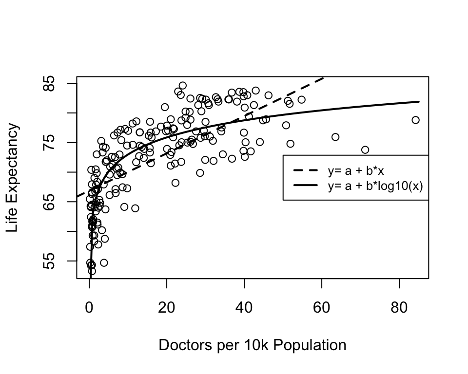
Figure 17.1: Alternative Models for the Relationship between Doctors per 10k and Life Expectancy
Note that the curved, solid line fits the data points much better than the straight, dashed line, which is what we expect based on the relative performance of the two regression models above. The interpretation of the curvilinear relationship is a bit different than that for the linear relationship. Rather than concluding that life expectancy increases as doctors per capita increases, we see in the scatterplot that life expectancy increases substantially as we move from nearly 0 to 14 or so doctors per 10,000 people, but increases beyond that point have less and less impact on life expectancy.
This is illustrated further below in Figure 17.2, where the graph on the left shows the relationship between docs10k among countries below the median level (14.8) of doctors per 10,000 population and the graph on the right shows the relationship among countries with more than the median level of doctors per 10,000 population. This is not quite as artful as Figure 17.1 with the plotted curved line, but it does demonstrate that the main gains from increased access to health care come at the low end of the scale, in this case countries with severely limited access (many countries have less than one doctor per 10,000 population). For the upper half of the distribution, there is almost no relationship between docs10k and life expectancy.
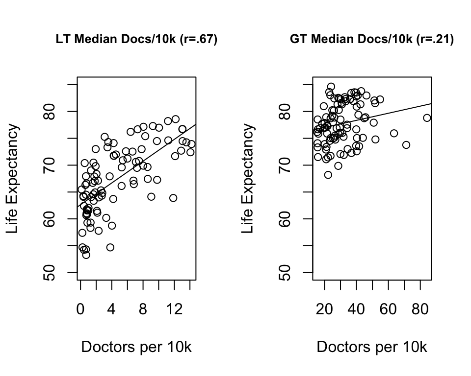
Figure 17.2: A Segmented View of a Curvilinear Relationship
Finally, we can re-estimate the multiple regression model with the appropriate version of docs10k to see if this transformation has an impact on its statistical significance.
#Re-estimate five-variable model using "log10(docs10k)"
fit<-lm(countries2$lifexp~countries2$fert1520 + countries2$mnschool+
          log10(countries2$pop) +countries2$urban+
          log10(countries2$docs10k),na.action = na.exclude)
#Using information in 'fit' to create a table of results
stargazer(fit, type="text", dep.var.labels=c("Life Expectancy"),
          covariate.labels = c("Fertility Rate","Mean Years of Education",
                               "Log10(Population)",
                               "% Urban","log10(Doctors per 10k)"))
===================================================
                            Dependent variable:
                        ---------------------------
                              Life Expectancy
---------------------------------------------------
Fertility Rate                   -2.810***
                                  (0.399)

Mean Years of Education           0.356**
                                  (0.163)

Log10(Population)                  0.050
                                  (0.329)

% Urban                          0.045***
                                  (0.015)

log10(Doctors per 10k)            2.420**
                                  (0.973)

Constant                         72.100***
                                  (2.130)

---------------------------------------------------
Observations                        179
R2                                 0.772
Adjusted R2                        0.765
Residual Std. Error          3.580 (df = 173)
F Statistic              117.000*** (df = 5; 173)
===================================================
Note:                   *p<0.1; **p<0.05; ***p<0.01
Accounting for the curvilinear relationship between docs10k and life expectancy made an important difference to the model. First, we now see a statistically significant impact from the logged version of the docs10k, whether using a one- or two-tailed test (the t-score changes from 1.83 in the original model to 2.49 in the model above). We need to be a little bit careful here when discussing the coefficient for the logged variable. Although there is a curvilinear relationship between docs10k and life expectancy, there is a linear relationship between log10(docs10k) and life expectancy. So, we can say that for every unit increase in the logged value of docs10k, life expectancy increases by 2.4 years, but we need to keep in mind that when we translate this into the impact of the original version of docs10k, the relationship is not linear. In addition to doctors per 10,000 population, the fertility rate and percent urban are also statistically significant (one-tailed test), and there is less error in predicting life expectancy when using the logged version of docs10k: the RMSE dropped from 3.606 to 3.577, and the R2 increased from .768 to .771.
17.4.1 Stop and Think
These findings underscore the importance of thinking hard about results that don’t make sense. There is a strong theoretical reason to expect that life expectancy should be higher in countries where there are more doctors per capita, as there is greater access to health care in those countries than in countries with fewer doctors per capita. However, the initial regression results suggested that doctors per capita was tangentially related to life expectancy. Had we simply accepted this result, we would have come to an erroneous conclusion. Instead, by exploring explanations for the null finding, we were able to uncover a more nuanced and powerful role for the number of doctors per 10k population. Of course, it is important to point out that one of the sources of “getting it wrong” in the first place was skipping a very important first step: examining the bivariate relationship closely, using not just the correlation coefficient but also the scatterplot. Had we started there, we would have understood the curvilinear nature of the relationship from the get go.
17.5 Which Variables have the Greatest Impact?
As a researcher, one thing you’re likely to be interested in is the relative impact of the independent variable; that is which variable has the greatest and least impact on the dependent variable? If we look at the regression slopes, we might conclude that the order of importance runs from highest-to-lowest in the following order: The fertility rate (b=-2.81) and log of doctors per 10k (b=2.42) most important and of similar magnitude, followed by education level in distant third (b=.36), followed by log of population (b=.05) and percent urban (b=.045), neither one of which seem to matter very much. But this rank ordering is likely flawed due to differences in the way the variables are measured. A tip off that something is wrong with this type of comparison is found in the fact that the slopes for urban population and the log of population size are of about the same magnitude, even though the slope for urban population is statistically significant (p<.01) while the slope for population size is not and has not been significant in any of the analyses shown thus far. How can a variable whose effect is not distinguishable from zero have an equal impact to one that has had a significant relationship in all of the examples shown thus far? Seems unlikely.
Generally, the “raw” regression coefficients are not a good guide to the relative impact of the independent variables because the variables are measured on different scales. Recall that the regression slopes tell us how much Yyis expected to change for a unit change in x. The problem we encounter when comparing these slopes is that the units of measure for the independent variables are mostly different from each other, making it very difficult to compare the “unit changes” in a fair manner.
Just to give you a sense of the impact of measurement scale on the size of the regression slope, consider the two plots below. Both plots show the relationship between the size of the urban population and country-level life expectancy. The plot on the left uses the percentage of a country’s population living in urban areas, and the plot on the right uses the proportion of a country’s population living in urban areas. These are the same variable, just using different scales. As you can see, other than the metric on the horizontal axis, both plots are identical. In both cases, there is a moderately strong positive relationship (r= .59): as the urban population increases in size, life expectancy also increases. But look at the linear equations that summarize the results of the bi-variate regression models. The slope for the urban population variable in the second model model is 100 times the size of the slope in the first model, not because the impact is 100 times greater but because of the difference in the scale of the two variables. This is the problem we encounter when comparing regression coefficients across independent variables measured on different scales.
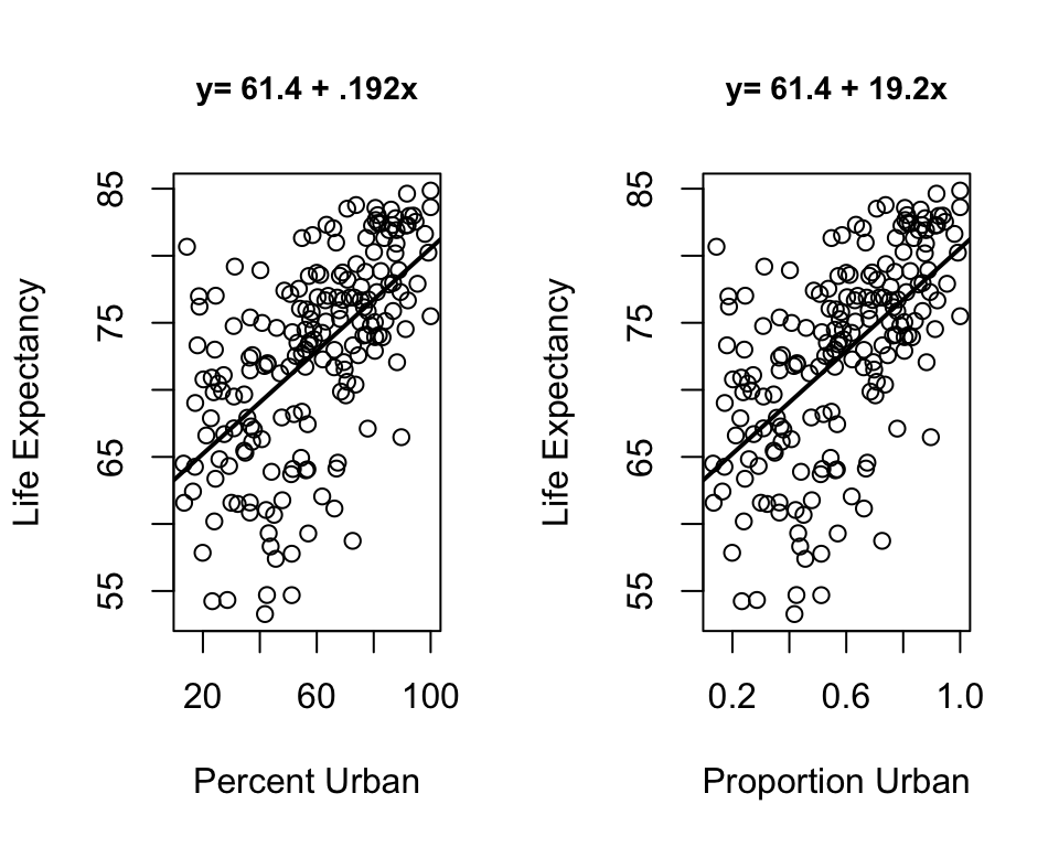
Figure 17.3: The Impact of Scale of the Independent Variable on the Size of Regression Coefficients
What we need to do is standardize the variables used in the regression model so they are all measured on the same scale. Variables with a common metric (same mean and standard deviation) will produce slopes that are directly comparable. One common way to standardize variables is to transform the raw scores into z-scores:
\[Z_i=\frac{x_i-\bar{x}}{S}\]
All variables (including the dependent variable) transformed in this manner will have \(\bar{x}=0\) and \(S = 1\). If we do this to all variables, we can get the standardized regression coefficients (sometimes confusingly referred to as “Beta Weights”). Fortunately, though, we don’t have to make these conversions ourselves since R provides the standardized coefficients for us. In order to get this information, we can use the StdCoef command from the DescTools package. The command is then simply StdCoef(fit), where “fit” is the object with the stored information from the linear model.
                          Estimate* Std. Error*  df
(Intercept)                 0.00000      0.0000 173
countries2$fert1520        -0.48092      0.0684 173
countries2$mnschool         0.15011      0.0687 173
log10(countries2$pop)       0.00567      0.0371 173
countries2$urban            0.13908      0.0471 173
log10(countries2$docs10k)   0.20610      0.0827 173
attr(,"class")
[1] "coefTable" "matrix"
The standardized coefficients are in the “Estimate” column. To evaluate relative importance, ignore the sign of the coefficient and only compare the absolute values. Based on the standardize coefficients, the ordering of variables from most-to-least in importance is a bit different than when we used the unstandardized coefficients: fertility rate (-.48) far outstrips all other variables, having more that twice the impact as doctors per 10,000 (.21), which is followed pretty closely level of education (.15) and urban population (.14), and population size comes in last (.006). These results give a somewhat different take on relative impact than if we relied on the raw coefficients.
We can also make more literal interpretations of these slopes. Since the variables are all transformed into z-scores, a “one unit change” in x is always a one standard deviation change in x. This means that we can interpret the standardized slopes as telling how many standard deviations y is expected to change for a one standard deviation change in x. For instance, the standardized slope for fertility (-.48) tells us that for every one standard deviation increase in the fertility rate we can expect to see a .48 standard deviation decline in life expectancy. Just to be clear, though, the primary utility of these standardized coefficients is to compare the relative impact of the independent variables.
17.6 Statistics vs. Substance
The model we’ve been looking at explains about 77% of the variation in country-level life expectancy using five independent variables. This is a good model fit, but it is possible to account for a lot more variance with even fewer variables. Take, for example, the alternative model below, which explains 99% of the variance using just two independent variables, male life expectancy and maternal mortality.
#Alternative model
fit1<-lm(countries2$lifexp~countries2$malexp + countries2$infant_mort)
#Table with results from both models
stargazer(fit, fit1, type="text",
          dep.var.labels=c("Life Expectancy"),
          covariate.labels = c("Fertility Rate",
                               "Mean Years of Education",
                               "Log10(Population)",
                               "% Urban",
                               "log10(Doctors per 10k)",
                               "Male Life Expectancy",
                               "Infant Mortality"))
===========================================================================
                                        Dependent variable:
                        ---------------------------------------------------
                                          Life Expectancy
                                  (1)                       (2)
---------------------------------------------------------------------------
Fertility Rate                 -2.810***
                                (0.399)

Mean Years of Education         0.356**
                                (0.163)

Log10(Population)                0.050
                                (0.329)

% Urban                         0.045***
                                (0.015)

log10(Doctors per 10k)          2.420**
                                (0.973)

Male Life Expectancy                                      0.810***
                                                          (0.018)

Infant Mortality                                         -0.081***
                                                          (0.007)

Constant                       72.100***                 17.400***
                                (2.130)                   (1.410)

---------------------------------------------------------------------------
Observations                      179                       184
R2                               0.772                     0.989
Adjusted R2                      0.765                     0.989
Residual Std. Error         3.580 (df = 173)          0.787 (df = 181)
F Statistic             117.000*** (df = 5; 173) 8,098.000*** (df = 2; 181)
===========================================================================
Note:                                           *p<0.1; **p<0.05; ***p<0.01
We had been feeling pretty good about our model that explains 77% of the variance in life expectancy, and then along comes this much simpler model that explains almost 100% of the variation. Not that it’s a contest, but this does sort of raise the question, “Which model is best?” The new model definitely has the edge in measures of error: the RMSE is just .787, compared to 3.577 in the five-variable model, and as mentioned above, the R2=.99.
So, which model is best? Of course, this is a trick question. The second model provides a stronger statistical fit but at significant theoretical and substantive costs. Put another way, the second model explains more variance without providing a useful or interesting substantive explanation of the dependent variable. In effect, the second model is explaining life expectancy with other measures of life expectancy. Not very interesting. Think about it like this. Suppose you are working as an intern at the World Health Organization and your supervisor asks you to give them a presentation on the sources of life expectancy around the world. How impressed do you think they would be if you came back to them and said you had two main findings:
- People live longer in countries where men live longer.
- People live longer in countries where fewer people die really young.
Even with your impressive R2 and RMSE, your supervisor would likely tell you to go back to your desk, put on your thinking cap, and come up with a model that provides a stronger substantive explanation, something more along the lines of the first model. With the results of the first model you can report back that two factors that are most strongly related to life expectancy across countries are fertility rates and access to health care, as measured by the number of doctors per 10k population. The share of the population living in urban areas is also related to life expectancy, but this is not something that can be addressed through policies and aid programs. The fertility rate and access to health care, however, are things that policies and aid programs might be able to affect.
17.7 Next Steps
By now, you should be feeling comfortable with regression analysis and, hopefully, seeing how it can be applied to many different types of data problems. The last step in this journey of discovery is to examine some of the important assumptions that underlie the OLS regression. In the Chapter 18, I provide a brief overview of assumptions that need to be satisfied in order to be confident in the results of the life expectancy model presented above. As you will see, in some ways, the model does a good job of satisfying the assumptions, but in other ways, the model still needs a bit of work. It is important to be familiar with these assumptions not just so you can think about them in the context of your own work, but also so you can use this information to evaluate the work of others.
17.8 Assignments
17.8.1 R Problems
Building on the regression models from the last chapter, use the states20 data set and run a multiple regression model with infant mortality (infant_mort) as the dependent variable, and per capita income (PCincome2020), the teen birth rate (teenbirth), percent low birth weight births lowbirthwt, and south as the independent variables.
Produce a publication-ready table using
stargazer. Make sure you replace the R variables names with meaningful labels (see Chapter 16 for instructions on doing this usingstargazer).Summarize the results of this model. Make sure to address matters related to the effects of the independent variables and how well the group of variables do in accounting for state-to-state differences in infant mortality.
Run the necessary test to standardized regression coefficients. Discuss the results. Any surprises? Make it clear that you understand why you need to run this test what these results are telling you.
Run a test for evidence of multicollinearity. Discuss the results. Any surprises? Make it clear that you understand why you need to run this test what these results are telling you.
Generate predicted values from the regression equation, plot the predicted against the observed values, and use state abbreviations (
stateab) to label each data point. Also include the regression line. Discuss the fit of the model, as revealed in the dispersion of the data points around the regression line, and make sure to highlight and discuss any states that you think stand our as possible outliers.
The number of missing cases is reported in the standard R output (not
stargazer) as “16 observations deleted due to missingness.”↩︎