Chapter 17 Introduction to big data analytics
17.1 Introduction
Previous chapters looked into traditional or classic data analysis: inference about a population using a limited sample of data with a limited number of variables. For instance, we might be interested in how large the effect is of a new kind of therapy for clinical depression in the population of all patients, based on a sample of 150 treated patients and 150 non-treated patients on a waiting list.
In many contexts, we are not interested in the effect of some intervention in a population, but in the prediction of events in the future. For example, we would like to predict which patients are likely to relapse into depression after an initially successful therapy. For such a prediction we might have a lot of variables. In fact, more variables than we could use in a straightforward linear model analysis.
In this age of big data, there are more often too many data then too few data about people. However, this wealth of data is often not nicely stored in data matrices. Data on patients for example are stored in different types of files, in different file formats, as text files, scans, X-rays, lab reports, perhaps even videotaped interviews. They may be stored at different hospitals or medical centres, so they need to be linked and combined without mixing them up. In short: data can be really messy. Moreover, data are not variables yet. Data science is about making data available for analysis. This field of research aims to extract knowledge and insight from structured and unstructured data. To do that, it draws from statistics, mathematics, computer science and information science.
The patient data example is a typical case of a set of unstructured data. From a large collection of pieces of texts (e.g., notes from psychiatric interviews and counselling, notes on prescriptions and adverse effects of medication, lab reports) one has to distil a set of variables that could predict whether or not an individual patient would fall back into a second depressive period.
There are a couple of reasons why big data analytics is different from the data analysis framework discussed in previous chapters. These relate to 1) different types of questions, 2) the \(p>n\) problem and 3) the problem of over-fitting.
First, the type of questions are different. In classic data analysis, you have a model with one or more model parameters, for example a regression coefficient, and the question is what the value is of that parameter in the population. Based on sample data, you draw inferences regarding the parameter value in the population. In contrast, typical questions in big data situations are about predictions for future data (e.g., how will the markets respond to the start of the hurricane season), or how to classify certain events (e.g., is a Facebook posting referring to a real event or is it "fake news"). In big data situations, such predictions or classifications are based on training data. In classic data analysis, inference is based on sample data.
Second, the type of data in big data settings allows for a far larger number of variables than in non-big data settings. In the patient data example, imagine the endless ways in which we could think of predicting relapse on the basis of the text data alone. We could take as predictor variables the number of counselling sessions, whether or not a tricyclic antidepressant was prescribed, whether or not a non-tricyclic antidepressant was prescribed, whether or not the word "mother" was mentioned in the sessions, the number of times the word "mother" was used in the sessions, how often the word "mother" was associated with the word "angry" or "anger" in the same sentence, and so on. The types of variables you could distil from such data is endless, so what to pick? And where to stop? So the first way in which big data analytics differs from classic data analysis is that a variable selection method has to be used. The analyst has to make a choice of what features of the raw data will be used in the analysis. Or, during the analysis itself, an algorithm can be used that picks those features that predict the outcome variable most efficiently. Usually there is a combination of both methods: there is an informed choice of what features in the data are likely to be most informative (e.g., the data analyst a priori believes that the specific words used in the interviews will be more informative about relapse than information contained in X-rays), and an algorithm that selects the most informative features out of this selection (e.g., the words "mother" and "angry"). One reason that variable selection is necessary is because statistical methods, like for example linear models, do not work when the number of variable is large relative to the number of cases. This is known as the \(p > n\) problem, where \(p\) refers to the number of variables and \(n\) to the number of cases. We will come back to this problem below.
Third, because there is so much information available in big data situations, there is the likely danger of over-fitting your model. Maybe you have enough cases to include 1,000 predictor variables in your linear models, and they will run and give meaningful output, but then the model will be too much focused on the data that you have now, so that it will be very bad at predicting or classifying new events correctly. Therefore, another reason for limiting the number of variables in your model is to prevent over-fitting. Limiting the number of variables in a model can be done by various variable selection methods, for example the LASSO in linear regression (Tibshirani, 1996). Over-fitting can also be countered by using so-called ensemble methods like boosting and random forest.
In order to check that you are not over-fitting, one generally splits the data into a training data set and a test data set (or validation data set). The training data are used to select the variables and fit the model (i.e., determine model parameters). For example, when a simple linear regression model is used to predict height in school children, the least squares estimates are determined based on the training data alone. Next, these estimates are used to predict new values for the test data. That is, we take the test data, use the predictor variables and plug them into the model equation and see what height values we predict for the children in the test data. Next, we compare these predicted values with the actually observed height measurements in these children. In the case of over-fitting, the model will show a very good fit (good predictions) to the training data but a poor fit to the test data (bad predictions). If there is no over-fitting, the predictions for the test data will not be much worse for the test data than for the training data.
As a small data example of the phenomenon of over-fitting, in Figure 17.1 we see a complete data set on variables \(X\) and \(Y\) for 30 observations. The actual relationship between the two variables can be described by a simple linear regression model \(Y = X + e\), where \(e\) has a normal distribution with standard deviation 10. But suppose we don’t know that, and we want to find a model that gives a good description for these data. We split the data set in half, and use a local polynomial regression fitting algorithm that best describes the training data. The training data set and the model predictions, depicted as a blue line is given in Figure 17.2. It turns out that the correlation between the observed \(Y\)-values and the predicted values based on the model is pretty high: 0.78.
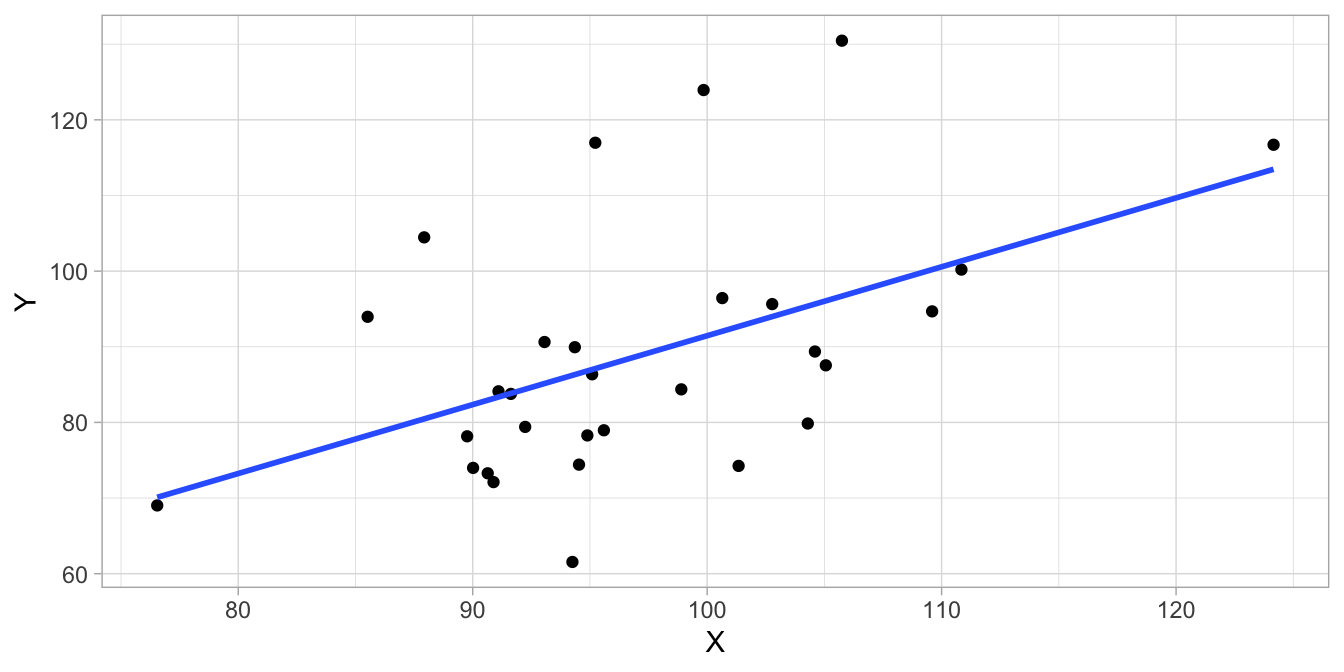
Figure 17.1: Illustration of overfitting: a data set showing all 50 data points showing a linear relationship between variables \(X\) and \(Y\).
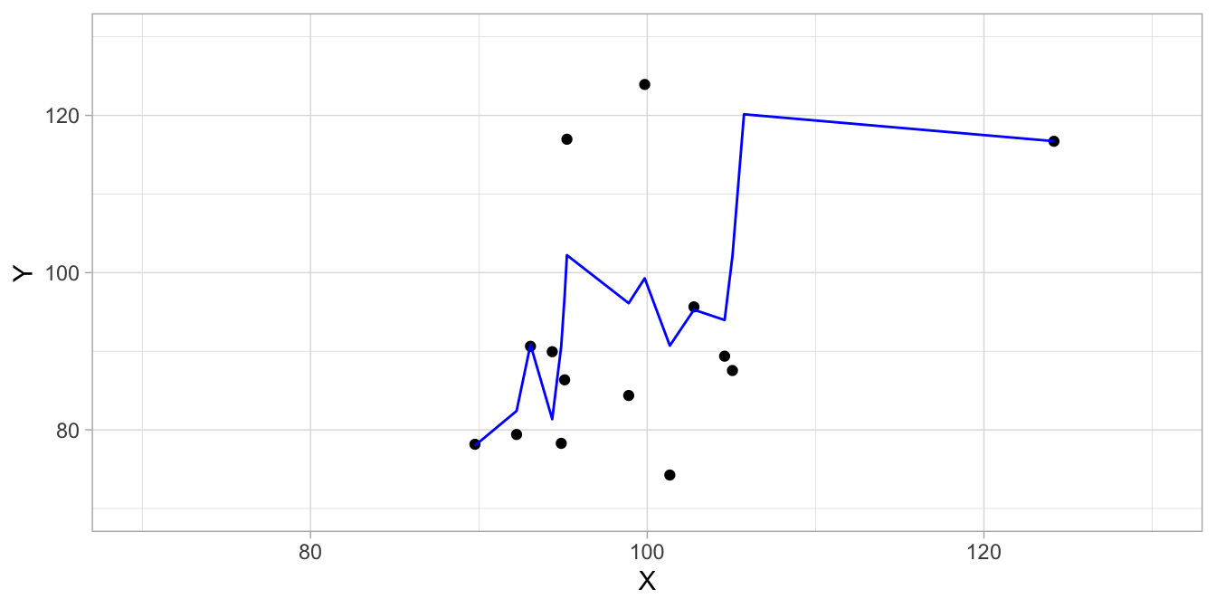
Figure 17.2: Illustration of overfitting: only showing half the data points (training data) and a local polynomial regression model fitted to them.
Next, we apply this model to the test data. These are depicted in Figure 17.3. The blue line are the predicted \(Y\)-values for the \(X\)-values in this data set, based on the model. We see that the blue line is not a good description of the pattern in the test data. This is also reflected in the much lower correlation between the observed \(Y\)-values and the predicted values in the test data: 0.71. Thus we see that the model is a good model for the training data, upon which the model was based, but the model is a terrible model for new data, even both data sets have the same origin. The training data were only randomly selected. The model was simply too much focused on the details in the data. Had we used a much simpler model, a linear regression model for example, the relative performance on the test data would be much better. The least squares equation predicts the \(Y\)-values in the training data with a correlation of 0.48. That is much worse than the splines, but we see that the model performs much better in the test data: there we see a correlation of 0.39. In sum: a complex model will always give better predictions than a simple model for training data. However, what is important is that a model will also show good predictions in test data. Then we see that often, a relatively simple model will perform better than a very complex model. This is due to the problem of over-fitting. The trade-off between the model complexity and over-fitting is also known as the bias-variance trade-off, where bias refers to the error that we make when we select the wrong model for the data, and variance refers to error that we make because we are limited to seeing only the training data.
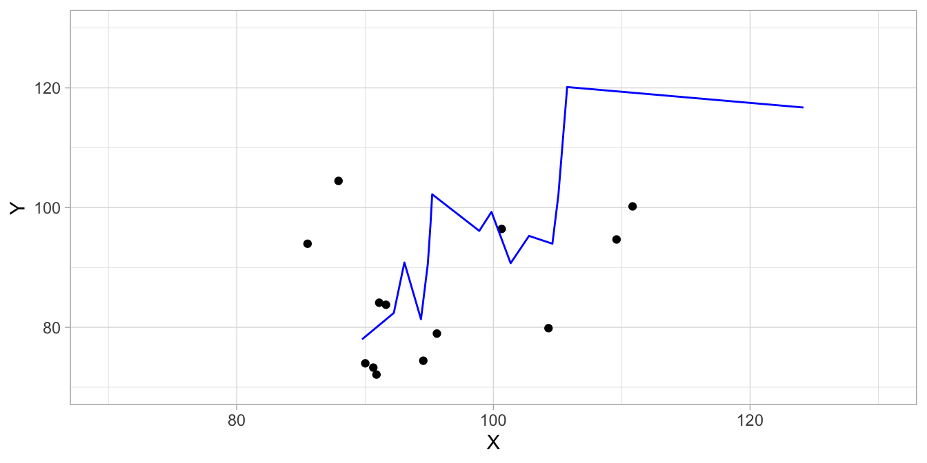
Figure 17.3: Illustration of overfitting: only showing half the data points (test data) and a local polynomial regression model that does not describe these data well because it was based on the training data.
17.1.1 Model selection
In the preceding chapters, we discussed only the linear model and the extensions thereof: the linear mixed model and the generalized linear model. In big data analytics one uses these models too, but in addition there is a wealth of other models and methods, too. To name but the most well-known: decision trees, support vector machines, smoothing splines, generalized additive models, naive Bayes, and neural networks. Each model or method in itself has many subversions. A very important part of big data analytics is therefore model selection. Models vary in their flexibility, that is, how well they can fit the data. Remember that when we looked at multiple regression, a model with many predictors usually shows a larger R-squared than a model with fewer predictors. That is, it explains or predicts the sample data better. But now we know that this also brings the danger of over-fitting: it fits the sample or training data better, but not necessarily the test data and the data that we want to predict in future applications. The same is true for simple models and more flexible models. A linear model with two additive predictors is a relatively simple model that might not explain so much variance in the training data. A neural network is an example of a very flexible model that might be much more able to capture variance in training data that shows a large amount of complexity, for example a complicated interaction pattern. We therefore have to make a trade-off between model flexibility and over-fitting that is dependent on each type of problem. If reality is complex we need a complex model to make the right predictions, but if reality is simple and we apply a complex model, we run the risk of over-fitting. If reality is complex and we use a simple model, we run the risk of bad predictions. In order to strike the right balance and find the optimal level of complexity for our training data, one often uses cross-validation.
17.1.2 Cross-validation
Cross-validation is a form of a re-sampling method. In re-sampling methods, different subsets of the training data are used to fit the same model or different models, or different versions of a model. There are different forms of cross-validation, but here we discuss \(k\)-fold cross-validation. In \(k\)-fold cross-validation, the training data are split randomly into \(k\) groups (folds) of approximately equal size. The model is then fit \(k\) times, each time leaving out the data from one of the \(k\) groups. Each time, predictions are made for the data in the group that is left out of the analysis. And each time we assess how good these predictions are, for example by determining the residuals and computing the mean squared error (MSE). With \(k\) groups, we then have \(k\) MSEs, and we can compute the mean MSE. If we do this cross-validation for several models, we can see which model has the lowest mean MSE. That is the model that on average shows the best prediction. This should not lead to over-fitting, because by the random sampling into \(k\) sub-samples, we are no longer dependent on one particular subset of the data. Usually, a value of 5 or 10 is used for \(k\).
17.1.3 The \(p>n\) problem
Suppose we have a data set consisting of 2 variables, \(X\) and \(Y\), with 3 observations. This data set is tabulated in Table 17.1. So we have \(n = 3\) and \(p = 2\). If we plot the data and fit a regression line with the least squares criterion, we encounter no problem, see Figure 17.4. This is because \(p\) is smaller than \(n\). Now let’s see what happens when \(p\) and \(n\) are of equal size. Suppose we omit the first observation and plot only the second and third observations. These are plotted in Figure 17.5. If we now fit a line using the least squares criterion, we see that we can only fit a line without residuals: the line shows a perfect fit. You can probably imagine that for any two data points, a linear line will always show a perfect fit without residuals. The variance of the residuals will be 0. The software that you use for fitting such a model will give you some sort of warning. R will say that there are no residual degrees of freedom. SPSS will say nothing special but will also show a 0 for the number of residual degrees of freedom. More obviously, the output will give you an intercept and a slope, but there will be no standard errors, and hence no \(t\)-values and no \(p\)-values. Therefore, you can say something about the intercept and slope in the sample, but you cannot say anything about the intercept and slope in the population.
| X | Y |
|---|---|
| 0 | 0.64 |
| 1 | 2.08 |
| 2 | 3.33 |
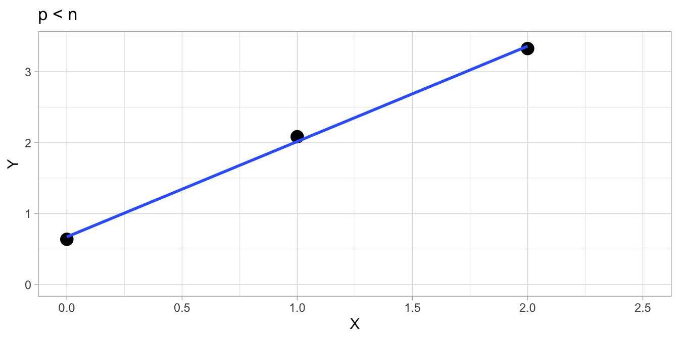
Figure 17.4: \(p < n\): There is a unique solution that fits the least squares criterion. No problem whatsoever.
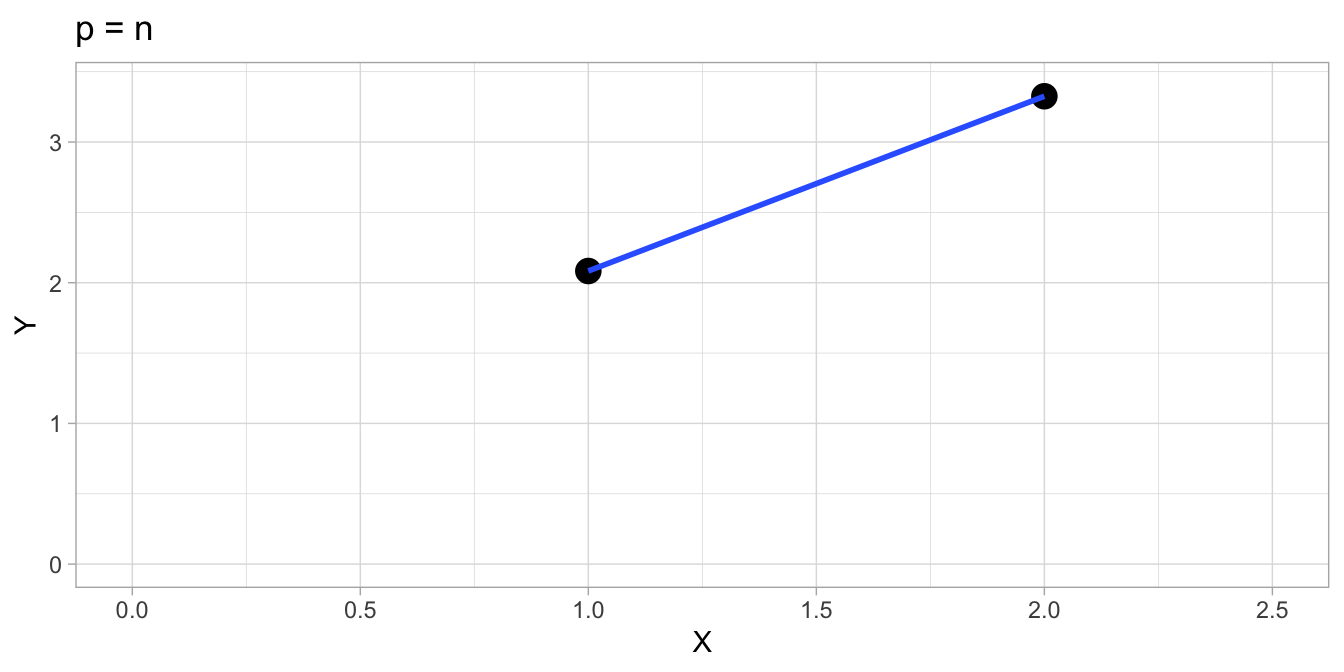
Figure 17.5: \(p = n\): There is a unique solution, but there are no degrees of freedom left. Standard errors cannot be determined, so no inference regarding the population parameters is possible.
The situation will be even worse when you have only 1 data point. Suppose we only have the second data point, which we plot in Figure 17.6. If we then try to fit a regression line, we will see that the software will refuse to estimate a slope parameter. It will be fixed to 0, so that an intercept only model will be fitted (see Section @ref(#sec:intercept-only)). It simply is impossible for the software to decide what regression line to pick that goes through this one data point: there is an infinite number of regression lines that go through this data point! Therefore, for a two-parameter model like a regression model (the two parameters being the intercept and slope), you need at least two data points for the model to run, and at least three data points to get standard errors and do inference.
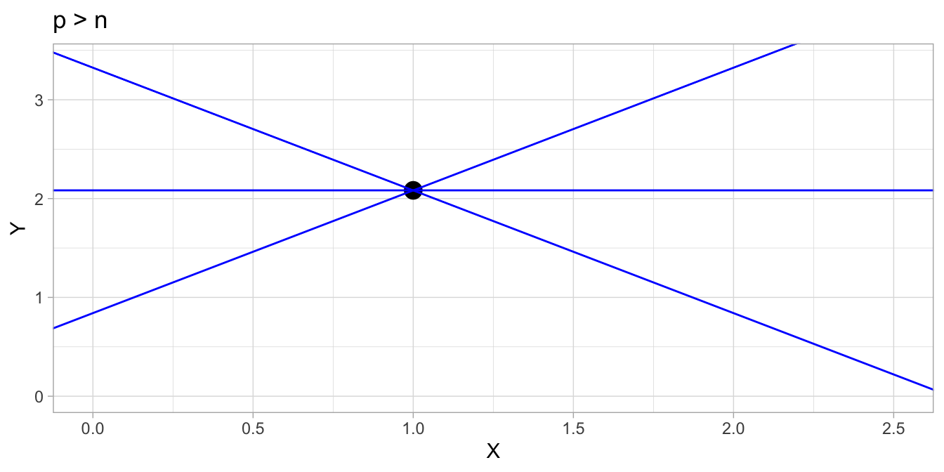
Figure 17.6: \(p > n\): There is an infinite number of lines through the data point, but there is no criterion that determines which is best. The problem of the least squares regression line is not defined with only one data point.
The same is true for larger \(n\) and larger models. For example, a multiple regression model with 10 predictor variables together with an intercept will have 11 parameters. Such a model will not give standard errors when you have 11 observations in your data matrix, and it will not run if you have fewer than 11 observations.
In sum, the number of data points, \(n\), should always exceed the number of parameters in your model. That means that if you have a lot of variables in your data file, you cannot always use them in your analysis, because you simply do not have enough rows in your data matrix to estimate the model parameters.
17.1.4 Steps in big data analytics
Now that we are familiar with the differences between classical data analysis and big data analytics and the major concepts, we can look at how all the elements of big data analytics fit together. In big data problems, we often see the following steps:
Problem identification. You need to know what the problem is: what do you want to know? What do you want to predict? How good does the prediction have to be? How fast does it have to be: real-time?
Selection of data sources. Depending on what you want to know or predict, you have to think about possible sources of information. Are there any websites that already contain part of the information that you are looking for? Are there any databases you can get access to?
Feature selection. From the data sources you have access to, what features are of interest? For example, from spoken interviews, are you mainly interested in the words spoken by the patient? Or perhaps interested in the length of periods of silence, or perhaps in changes in pitch? There are so many features you could extract from data.
Construction of a data matrix. Once you have decided what features you want to extract from the raw data, you have to put this information into a data matrix. You have to decide what to put in the rows (your units of observation), and in the columns (the features, now variables). So what is now your variable: this could be the length of one period of silence within one interview for a particular patient. But it could also be the average pitch for a 1-minute interval in one interview for one particular patient.
Training and test (validation) data set. In order to check that we are not over-fitting, and to make sure that our model will work for future data, we divide our data set (our data matrix) into two parts: training data and test data. This is done by taking a random sample of all the data that we have. Usually, a random sample of 70% is used for training, and the remaining 30% is used for testing (validating) the model. We set the test data aside and will only look at the training data.
Model selection. In data science it is very common to try out various models or various sub-models on the training data to see which model fits the data best. To make sure that we do not over-fit the data, we use some form of cross-validation, where we split up the training data even further.
Build the model. Once we know what model works best for our training data, we fit that model on the training model. This fitted model is our final model.
Validate the model. The final test is whether this final model will work on new data. We don’t have new data, but we have put away some of our data as test data (validation data). These data can now be used as a substitute for new data to estimate how well our model will work with future data.
Interpret the result and evaluate. There will be always some over-fitting, so the performance on the test data will always be worse than on the training data. But is the performance good enough to be satisfied with the model? Is the model useful for daily practice? If not, maybe the data sources and feature selection steps should be reconsidered. Another important aspect of statistical learning is interpretability. There are some very powerful models and methods around that are capable of very precise predictions. However, the problem with these models and methods is that they are hard to interpret: they are black boxes in that they make predictions that cannot be explained by even the data analysts themselves. Any decisions are therefore hard to justify, which brings ethical issues. For instance, what would you say if an algorithm would determine on the basis of all your life’s data that you will not be a successful student? Of course you would want to know on the basis of what data exactly that decision is based. Your make-up? Your height? The colour of your skin? Last year’s grades? Of course it would matter to you what variables are used and how. Recent research has focused on how to make complicated models and methods easier to interpret and help data analysts evaluate the usefulness and applicability of their results and communicate them to others.