

| 0 | 1 | 2 | 3 | 4 | 5 | 6 | 7 | 8 | 9 | 10 |
|---|---|---|---|---|---|---|---|---|---|---|
| 303 | 42 | 172 | 270 | 369 | 1281 | 853 | 1344 | 1295 | 353 | 356 |
Seminar: Kausalanalyse
Ein Einsteiger-Seminar für Studierende der Politikwissenschaft
Updated: Jul 17, 2024
Session 1
Introduction
Introduction
When, where, requirements, contact, grading: See syllabus
Document for posting questions can be found here.
Content of slides is a fusion of…
- …book project Applied Causal Analysis & Machine Learning (with R) (with Denis Cohen, Lion Behrens)
- …past lectures & seminars (Kreuter, Bach, Bauer etc.) (e.g., applied causal analysis seminar)
- …different books, articles and material from different disciplines (see citations)
Sociology of research methodology (Where did you study?)
Session 2
Statistical foundations: Measurement, variables, data (distributions) and models
Today’s objectives
- Discuss components of a research design & definition
- Research questions, hypotheses, population & sampling method, conceptualization & measurement, observations & data
- Terminfindung: https://forms.gle/Sdtj2fj9U1hzoev37
![]()
Research design: Definition
- Wikipedia (careful!) on research design (RD)
- A framework that has been created to find answers to research questions
- A set of methods and procedures used in collecting and analyzing measures of the variables specified in the research question
- Wrong RD → wrong answer to research question (RQ) → potentially drastic consequences (e.g., medicine)
- Bad RQs → bad RDs (e.g, RQ is too vague)
- Criteria for “good research design” change over years/decades
Replication crisis
- Replication crisis (Q: Retraction watch?) (Open Science Collaboration 2015)
- Reasons: Research design errors, fraud and coding errors (e.g., Psychoticism)
- What a massive database of retracted papers reveals about science publishing’s ‘death penalty’
- Increasing calls for open science to foster replicability and reproducability
- Terminology: Reproduction vs. replication
Research design: Components by Babbie (2015, 114)
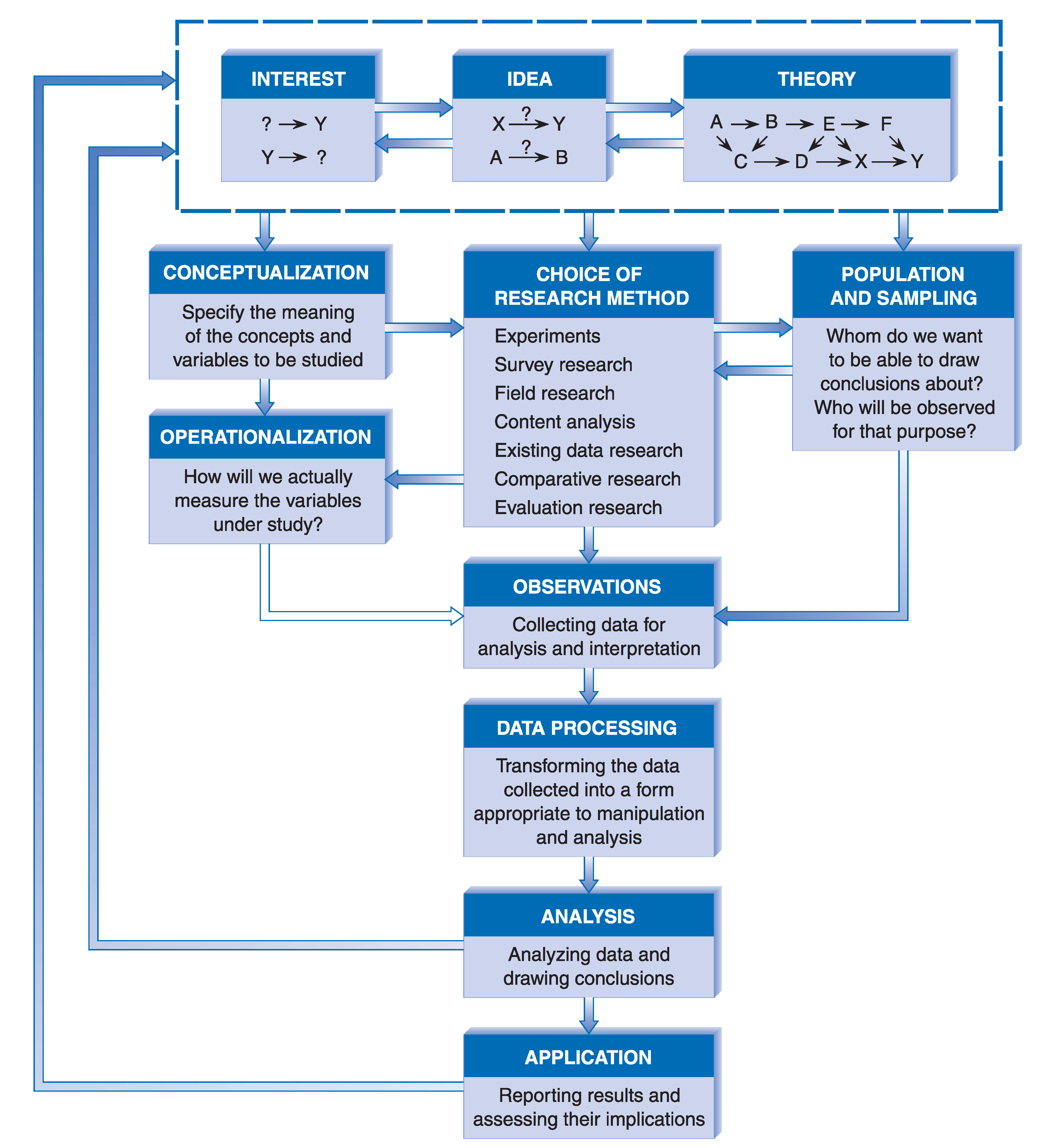
Research design (RD): Steps
- Formulate a research question and hypotheses
- Specify target population (e.g., humans) and sampling method (e.g., random sample)
- Specify concepts (conceptualization) and their measures (operationalization)
- Choose a research method, e.g., a randomized experiment
- Collect data or use data that has been collected (observations)
- Analyze data (statistical modelling)
- Important: Steps may overlap and order may change during research process (see Babbie’s graph)
Research questions: Types
- Empirical analytical (positive) vs. normative
- Should men and women be paid equally? Are men and women paid equally (and why?)?
- Q: Which one is empirical-analytical, which one normative? Can we derive hypotheses for normative questions?
- Y-based, X-based and y = f(x)-based (Plümper 2014, 22)
- Y-based: What causes differences in income (Y)?
- X-based: What are the consequences of differences in education (X), i.e., how does it impact other outcome variables?
- y = f(x)-based: Do differences in education (X) cause differences in income (Y)? (Gerring 2012, 646–48)
- What? vs. Why? (Gerring 2012, 722–23)
- Describe aspect of the world (What?) vs. causal arguments that hold that one or more phenomena generate change in some outcome (imply a counterfactual) (Why?)
- My personal preference: descriptive vs. causal questions vs. predictive questions
Research questions: Descriptive
Measure:‘Would you say that most people can be trusted or that you can’t be too careful in dealing with people, if 0 means “Can’t be too careful” and 10 means “Most people can be trusted”?’
RQ: What is the average level of trust (Y)? How are individuals distributed? (univariate)
- We can add as many variables/dimensions as we like (e.g. gender, time) → multivariate
- Q: What would the table above look like when we add gender as a second dimension?
- Descriptive questions (multivariate)
- RQ: Do females have more trust than males? (multivariate)
- RQ: Did trust rise across time?(multivariate)
Research questions: Causal
| 0 | 1 | 2 | 3 | 4 | 5 | 6 | 7 | 8 | 9 | 10 | |
|---|---|---|---|---|---|---|---|---|---|---|---|
| no victim | 259 | 36 | 135 | 214 | 320 | 1142 | 782 | 1228 | 1193 | 326 | 331 |
| victim | 44 | 6 | 37 | 56 | 48 | 139 | 70 | 114 | 101 | 27 | 25 |
- Descriptive RQs: Do victims have a different/lower level of trust from/than non-victims?
- Mean Non-victims: 6.2; Mean Victims: 5.48
- Why?-questions start with difference(s) and, then, seek to explain why those difference(s) occured
- Why does this group of people have a higher level of trust?
- Causal questions: Is there a causal effect of victimization on trust? (We’ll define causal effect later)
- Insights
- Data underlying descriptive & causal questions is the same
- Causal questions link Y to one (or more) explanatory causes X (or D)
Research questions: Precision
- Q: Below you find different versions of the same research question. What is the most precise question and why is it precise?
Is there a causal effect of victimization on trust in a sample of Swiss citizens?
What is the impact of negative experiences on trust?
Is there a causal effect of victimization on generalized trust in a sample of Swiss aged from 18 to 98 in 2010?
What is the impact of victimization on generalized trust?
Research questions → hypotheses
Hypotheses = expectations we have for the answers to our research question (descriptive or causal)
RQ: Does smoking increase the probability of/cause cancer?
- Q: What hypotheses could we formulate?
- Hypotheses:
- Smoking has an/no effect on the probability of getting cancer!
- Smoking has a positive effect on (increases the probability of) getting cancer! (the higher X, the higher Y)
- Smoking has a negative effect on (decreases the probability of) getting cancer! (the higher X, the lower Y)
Hypotheses: Precision (1)
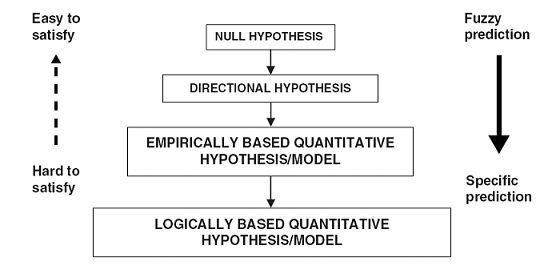
- Hypotheses are not created equal (Taagepera 2008, 71–81)
- Null hypothesis: Focus on “disproving that something is due to chance”
- Directional hypothesis: Hold that increasing X will increase or decrease Y (we are here…)
- Emp. based quant. hypothesis: Focusses on the shape of the function y = f(x) [Ceteris paribus]
- Log. based quant. hypothesis: Formal theoretical model that makes a prediction, i.e., generates a hypothesis
Hypotheses: Precision (2)
- Q: Which of the hypotheses below is a null/directional/emp. based quant. hypothesis?
- Smoking increases the probability of getting cancer by 1% per 100 cigarettes
- Smoking has an effect on the probability of getting cancer
- Smoking increases the probability of getting cancer
- Most social science research studies use null or directional hypotheses.
Research design (RD): Steps
- Formulate a research question and hypotheses
- Specify target population (e.g., humans) and sampling method (e.g., random sample)
- Specify concepts (conceptualization) and their measures (operationalization)
- Choose a research method, e.g., a randomized experiment
- Collect data/sample or use data that has been collected (observations)
- Analyze data (statistical modelling)
Population & sampling method (1)
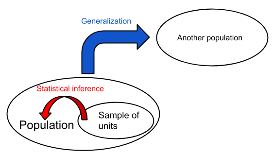
- Q: What do the concepts internal/external validity describe?
- Target population = Students at Freiburg university and Sample = students in this classroom
- Internal validity (Abadie et al. 2020): Is estimate = true (causal) effect in the sample (= students in this classroom) [requires random assignment]
- External validity (Abadie et al. 2020): Is estimate = value in the population (= Freiburg University students) [requires random sampling]
- Generalizability: e.g., generalize from sample (= students in this classroom) to.. ..other populations (e.g., LMU Munich students)? ..other times (e.g., Freiburg University students in 2027)? ..other settings (e.g., cinema)? Or a combination thereof.1
Population & sampling method (2)
Sampling: Select subset of units from population to estimate characteristics of that population
Steps: Researcher (we)…
- …define (target) population.
- …create a sampling frame = list of population members to sample from
- Q: Can you imagine a situation where population \(\neq / =\) sampling frame?
- …choose sampling method & units that should be in the sample.
Q: Are the above steps necessary when we work with secondary data (e.g., ALLBUS)?
- No.. but we should still evaluate representativeness (statistical inference).
Population & sampling method (3)
- Q: Imagine we are interested in estimating population averages/prop.. Below you find pairs of (target) population and sample: Are these good or bad samples? Why? Any bias?
- Income: Population: Freiburg university students; Sample: Students in this seminar
- Income: Population: Immigrants in Germany; Sample: Turkish immigrants
- Age: Population: Whatsapp users; Sample: Random sample of Whatsapp users
- Racist comments: Population: Tweets; Sample: Random sample of tweets provided by Twitter
- Q: What might be the problem with secondary data as opposed to data that you collect yourself?
Population & sampling method (4)
Population & sampling method (5)
Sampling techniques (Cochran 2007)
Simple random sampling: (1) Units in the population are numbered from 1 to N; (2) Series of random numbers between 1 and N is drawn; (3) Units which bear these numbers constitute the sample (ibid, 11-12) → Each unit has same probability of being chosen
Stratified random sampling: (1) Population divided into non-overlapping, exhaustive subpopulations (strata); (2) Simple random sample is taken in each stratum (ibid, 65f)
Quota sampling: Decide about N units that are wanted from each stratum (e.g., age, gender, state) and continue sampling until the neccessary “quota” has been obtained in each stratum (ibid, 105)
Snowball sampling: (1) Locate members of special population (e.g., drug addicts); (2) Ask them to name other members of population and repeat this step (Sudman and Kalton 1986, 413) → use snowballing to create sampling frame, then sample
- “Relaxed” version: Interview those named until sample size is reached
- Q: Does this create weaker or stronger bias? (ibid, 413)
- “Relaxed” version: Interview those named until sample size is reached
Research design (RD): Steps
- Formulate a research question and hypotheses
- Specify target population (e.g., humans) and sampling method (e.g., random sample)
- Specify concepts (conceptualization) and their measures (operationalization)
- Choose a research method, e.g., a randomized experiment
- Collect data or use data that has been collected (observations)
- Analyze data (statistical modelling)
Measurement & variables (1)
“the most important thing in statistics that’s not in the textbooks” (Gelman, April, 2015)
Theories (and the hypotheses they imply) (Moore and Siegel 2013, 3–4)
- Concern relationships among abstract concepts
- Variables are the indicators we use to measure our concepts
A [theoretical] variable has different theoretical “levels” or “values” (Jaccard and Jacoby 2019, 13)
- e.g., gender can be conceptualized as a variable that has two values (or more)
Empirical value of a variable for a given unit u (ui): the number assigned by some measurement process to u (Holland 1986, 954), e.g., male (0) or female (1)
Random variables: “If we have beliefs (i.e., probabilities) attached to the possible values that a variable may attain, we will call that variable a random variable.” (Pearl 2009, 8)
Measurement & variables (2): Quantifying the world
- Albert Einstein: “the whole of science is nothing more than an extension of everyday thinking” (Jaccard and Jacoby 2019, Ch. 2)
- Concepts (gender, education, race etc.) are the foundations stones of thinking in daily life & science

- Quantification = assignment of variable values to real-world objects
| id | gender | age | degree | subject |
|---|---|---|---|---|
| John | M | 25 | bachelor | sociology |
| Petra | F | 30 | master | physics |
| Hans | M | 29 | master | biology |
- Social scientists identify and classify people, countries, etc. according to various concepts
Measurement & variables (3)
| names | id | gender | income | education | happiness | age |
|---|---|---|---|---|---|---|
| Hans | 1 | male | 1000 | 0 | 5 | 30 |
| Peter | 2 | male | 5000 | 3 | 10 | 30 |
| Julia | 3 | female | 500 | 1 | 3 | 30 |
| Andrea | 4 | female | 1600 | 3 | 7 | 30 |
| Feli | 5 | female | 1600 | 3 | 7 | 30 |
Columns = variables
Rows = observations (often observations = units but not always)
Q: Which type of dataset has more observations (rows) than units? (Tip: Pa…)
Q: What are the theoretical and observed (empirical) values of happiness and age?
Q: Which are constants and which are variables in the above data frame? What is the difference?
- Idea of constant relevant later on (holding things constant!)
Research design (RD): Steps
- Formulate a research question and hypotheses
- Specify target population (e.g., humans) and sampling method (e.g., random sample)
- Specify concepts (conceptualization) and their measures (operationalization)
- Choose a research method, e.g., a randomized experiment (next weeks!)
- Collect data or use data that has been collected (observations)
- Analyze data (statistical modelling) (next weeks!)
Data collection (1): Measurement error
- Q: What is measurement (or observational) error? Can you give an example?
- Difference between a measured value of a variable and its true value
- e.g., difference between Peter’s measured and his real income
- Q: What is random and systematic measurement error? Can you give an example?
Systematic error:
- If men systematically provide income values that are above the real values
- If victims systematically under-report their victimization (Me Too movement!)
Random error: In repeated measures, a scale randomly deviates from your true weight
Partly conceptual confusion around terms such as reliability, repeatability (Bartlett and Frost 2008) (Q: Validity? Reliability?)
Data collection (2): Meas. error example
.png)
- Q: Which colors does this dress have?
- Please give an answer: https://www.menti.com/msg5qk5bb4
- After the vote: What do you think will be the result?

Data collection (3): Meas. error example
- Q: What can we learn from this example? (intersubjective agreement)
Data collection (4): Meas. equivalence
- Concept: Left-right ideology; Survey measure: “In politics people sometimes talk of ‘left’ and ‘right’. Using this card, where would you place yourself on this scale, where 0 means the left and 10 means the right?” (ESS 2012)
- Q: What does the graph below illustrate? (Bauer et al. 2017, 558)
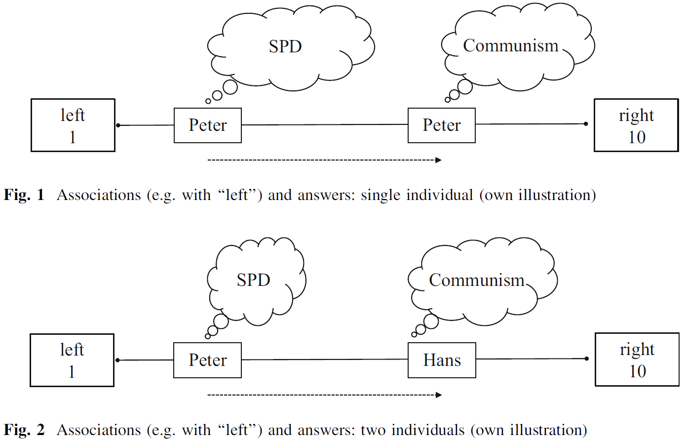
- Measurement inequivalence: When a measure provides different values for units with the same underlying true value, e.g., because of differential interpretation
Data (1)
After decisions about research question, population, sample, concepts, and measures we finally choose a research method and have collected data
Lecture focuses on causal inference using experimental/observational data so let’s quickly reiterate what data is!
Data: Units’ observed values on different variables (observations)
- Time is just another variable
Variables: Dimensions of the data space
Empirical observations are distributed across those dimensions, i.e., across (theoretical) values of those variables
Data (2)
- Data example: ‘Negative Experiences and Trust: A Causal Analysis of the Effects of Victimization on Generalized Trust’ (Bauer 2015)
- What is the causal effect of being victimized (= threatened) on trust?
- Population: People living in Switzerland
- Units: Individuals
- Data:
- Sample: 6633 Individuals (Switzerland!) (Sampling method)
- Variables: Victimization/Threat (0,1); Education (0-10) → Trust (0-10); Age (0-94)
- Time: data from 2006 (here)
- Q: How do we normally show/look at data?
Data: Table format
| Name | trust2006 | threat2006 | education2006 |
|---|---|---|---|
| Aseela | 4 | 0 | 8 |
| Dominic | 5 | 1 | 1 |
| Elshaday | 0 | 0 | 0 |
| Daniel | 5 | 0 | 9 |
| Sulaimaan | 7 | 0 | 4 |
| Peyton | 5 | 0 | 1 |
| Mudrik | 2 | 0 | 4 |
| Alexander | 7 | 0 | 5 |
| .. | .. | .. | .. |
- Q: How many rows should this table have if N = 6633? How many dimensions?
- Aseela[4, 0, 8]: Position of Aseela in the multi-dimensional space
Data: Univariate distribution(s)
| 0 | 1 | 2 | 3 | 4 | 5 | 6 | 7 | 8 | 9 | 10 |
|---|---|---|---|---|---|---|---|---|---|---|
| 303 | 42 | 172 | 270 | 368 | 1281 | 852 | 1342 | 1294 | 353 | 356 |
| 0 | 1 |
|---|---|
| 5966 | 667 |
| 0 | 1 | 2 | 3 | 4 | 5 | 6 | 7 | 8 | 9 | 10 |
|---|---|---|---|---|---|---|---|---|---|---|
| 380 | 806 | 194 | 89 | 2182 | 324 | 687 | 474 | 195 | 425 | 877 |
- Q: Where are most individuals located on the trust2006 and threat2006 variables?
Data: Joint distribution(s) [1]
Measures on several variables → multivariate joint distribution
3 variables: Victimization/Threat (0,1); Education (0-10) → Trust (0-10)
Q: How many dimensions? How many theoretical value combinations?
Data: Joint distribution(s) [2]
- Units are grouped on three variables: Trust (Y), Threat (D) and Education (X)
- Q: What would the corresponding dataset/dataframe look like?
- Q: What would a joint distribution with 4 variables look like?
- Q: What is a conditional distribution?
- Q: What does the joint distribution of two perfectly correlated variables look like?
- Important: Often we can only make a causal claims for a subset of our data (e.g., education = 4)
Data: One more joint distribution
Associational vs. causal inference
Joint distribution is basis for any quantitative analysis (Holland 1986, 948) of variables used in the design/analysis
Associational inference (descriptive questions, what?):
- Summarize joint distribution with statistical model (e.g., regression model)
- Does not tell us anything about causality, e.g., coefficient represents effect in both directions (Trust ↔︎ Threat)
Causal inference (causal questions, why?):
- Summarize joint distribution with statistical model (e.g., regression model)
- Add assumptions
- Give causal interpretation to coefficients!
Research design (RD): Steps with examples
- Formulate a research question and hypotheses
- RQ: Is there a causal effect of victimization on trust (Bauer 2015)?
- Hypothesis: Yes there is a positive effect!
- Specify target population (e.g., humans) and sampling method (e.g., random sample)
- Target population: Swiss population; Sampling method: Random sample of households
- Specify concepts (conceptualization) and their measures (operationalization)
- Define victimization & trust and choose survey questions
- Choose a research method, e.g., a randomized experiment (next weeks!)
- Use survey with repeated observations (panel data)
- Collect data or use data that has been collected (observations)
- Take data from the Swiss Household Panel (SHP)
- Analyze data (statistical modelling)
- Use matching + difference-in-differences
Quiz
- Please do the quiz under the link provided in the seminar.
Session 3 & 4
Causal analysis: Concepts and definitions
The causal inference ‘revolution(s)’
- Revolution of identification Keele (2015)
- Revolution of potential outcomes (Rubin 1974)
- Consequences
- New Style of writing/conducting data analysis
- New rationales for evaluating research (Causal empiricism)
- Has impacted research questions (search for natural experiments…)
- Exciting ongoing debates (e.g., on RCTs in development economics, Banerjee, Duflo, Deaton)
Causality everywhere!
- Many research questions (at least implicitly) aim to identify a causal effect
- Is there a causal effect of schooling on earnings/electoral participation?
- What is the effect of obtaining a master’s degree (compared to a bachelor’s degree) on lifetime earnings/vote choice?
- Should high school last eight or nine years?
- Does contact with migrants reduce xenophobic attitudes?
- Are gender-mixed teams more productive?
- Does survey question difficulty affect the quality/accuracy of responses?
- Does minimum wage affect employment?
- Are unemployed people less happy?
- Does unemployment benefits affect the health of recipients?
Causality & causes
- Some examples of causal statements
- My headache went away because I took an aspirin.
- Sarah earns a lot of money because she went to college.
- Tom found a job because he participated in a job training program.
- Revenues went up because firm X hired more people.
- Tomatoes are large this year because the summer was hot.
- Causality tied to
- an action
- taking an aspirin / going to college / job training program / hiring new people / a lot of sun (“conceptually”)
- applied to a unit
- me / Sarah / Tom / firm / tomatoes
- an action
Cause = action
- Causality tied to action applied to unit at particular point in time (Imbens and Rubin 2015, 4)
- An action (in our case binary)
- Action / No action
- Action A / Action B
- Often called treatment / control
- Easily extendable to multiple actions
- Action A / Action B / Action C
- Action A / Action B / Action C / No action
- Unit: Pretty much anything… a person, a group, any physical object
- Time: The same unit at a different time is a different unit (Imbens and Rubin 2015)
- Better: different observation of the same unit
Potential outcomes & causal effect
Given an unit (individual/you!) and a set of actions (take aspirin or not) we associate each action-individual pair with a potential outcome
Example (Peter has a headache): Aspirin (0 = no/1 = yes) → headache/Kopfschmerzen (0 = no/1 = yes)
- Potential outcome 1: Peter’s headache when taking aspirin
- Potential outcome 2: Peter’s headache when not taking aspirin
Definition individual-level causal effect
Difference in potential outcomes, same individual, same moment in time post-treatment (Imbens and Rubin 2015)
Causal effect = treatment effect
Individual causal/treatment effect
- Treatment variable \(D\): Aspirin
- \(D_{i}\): Value of \(D\) for individual \(i\) (1 = aspirin = treatment, 0 = no aspirin = control)
- Outcome variable \(Y\): Headache
- \(Y_{i}(\color{red}{1})\), \(Y_{i}(\color{blue}{0})\): Potential outcomes for individual \(i\)
- e.g., \(Y_{i}(\color{red}{1})\): Headache Peter would have when taking an aspirin
- \(Y_{i}\): Realized outcome → Headache we observe
- \(Y_{i}(\color{red}{1})\), \(Y_{i}(\color{blue}{0})\): Potential outcomes for individual \(i\)
- Individual-level Treatment Effect (ITE)
\(ITE = Y_{i}(\color{red}{1}) - Y_{i}(\color{blue}{0})\) ( \(t\) often omitted)
\(ITE_{Peter} = \text{Headache}_{Peter}(\color{red}{\text{Aspirin}}) - \text{Headache}_{Peter}(\color{blue}{\text{No aspirin}})\)
Fundamental problem of causal inference (Holl. 1986)
- Only one potential outcome will ever be realized and observed!
- Unobserved potential outcome also called counterfactual outcome
- Let’s assume Peter takes an aspirin \(D_{Peter} = 1\)
- We observe \(Y_{Peter}(\color{red}{1})\) but not \(Y_{Peter}(\color{blue}{0})\)
- Then we have the following data:
| \(\quad i\quad\) | \(\quad D_i\quad\) | \(\quad Y_{i}\quad\) | \(\quad Y_{i}(\color{red}{1})\quad\) | \(Y_{i}(\color{blue}{0})\) |
|---|---|---|---|---|
| Peter | 1 | 0 | 0 | ? |
- But we can not calculate \(ITE_{Peter} = Y_{Peter}(\color{red}{1}) - Y_{Peter}(\color{blue}{0}) = 0 - ?\)
Solution?
Missing data problem: We don’t observe the missing potential outcome
- here \(Y_{i}(\color{blue}{0})\), potential outcome under control is missing
| \(\quad i\quad\) | \(\quad D_i\quad\) | \(\quad Y_{i}\quad\) | \(\quad Y_{i}(\color{red}{1})\quad\) | \(Y_{i}(\color{blue}{0})\) |
|---|---|---|---|---|
| Peter | 1 | 0 | 0 | ? |
- Q: What is the solution? What could we fill in for missing value? Compare Peter with…?
- Q: What kind of person would you choose as a comparison for Peter?
Estimation of causal effects
- Missing data problem:
- Calculating treatment effect requires filling in missing counterfactual outcome
- Two solutions
- Either compare Peter to someone else
- e.g., Peter’s headache with Hans’s who did not take an aspirin (“social twin”)
- Between-individual comparative strategy (requires multiple units)
- Or compare Peter to himself
- e.g., Peter’s headache with his headache before taking the aspirin
- Within-individual comparative strategy
- Either compare Peter to someone else
- In making such comparisons we rely on assumptions, e.g., “unit homogeneity” (Holland 1986, 948)
Assumptions: Scientific solution
- unit homogeneity (Holland 1986, 948): Compare two different units and assume they are the same (e.g., 2 samples of substance in lab)
- temporal stability (a) and causal transience (b) (Holland 1986, 948): Measure causal effect by sequential exposure of unit \(i\) to control and then to treatment, measuring \(Y\) after each exposure
- states that the outcome value for unit \(i\) under control, does not depend on when the sequence ‘apply control to unit \(i\) then measure \(Y\) on \(i\)’ occurs
- i.e., Peter’s value under control would be the same regardless of when Peter is assigned to the control condition
- states the outcome value of unit \(i\) under treatment is not affected by the prior exposure of \(i\) to the sequence in (a)
- Peter’s value under treatment not affected by control condition and measurement of \(Y\) beforehand
- Scientific solution (exploit assumptions above) vs. statistical solution (average causal effect = expected value of the differences) (Holland 1986, 947)
Quick summary
Definition of causal effect does not require more than one individual (Imbens and Rubin 2015, 8)
- Difference in potential outcomes, same individual, same moment in time post-treatment
- \(ITE_{Peter} = \text{Headache}_{Peter}(\color{red}{\text{Aspirin}}) - \text{Headache}_{Peter}(\color{blue}{\text{No aspirin}})\)
BUT only one potential outcome realized (and observable)
Estimation: Pursue between-individual comparisons or within-individual comparisons
Individuals = units = can be anything (school classes, firms, governments etc.)
Q: How many potential outcomes do we have for a treatment variable Aspirin (no/yes), Education (primary school/high school/university) and Motivation (lowest/low/high/highest)?
Exercise: Vague actions & potential oucomes
- Sometimes, it is difficult to clearly define actions and potential outcomes
- Q: What is the action, what are the potential outcomes?
- My headache went away because I took an aspirin
- Sarah earns a lot of money because she went to college.
- Tom found a job because he participated in a job training program.
- Firm X’s revenues went up because it hired more people.
- Tomatoes are large this year because the summer was hot.
- …
- Tom was promoted because he is a man.
- The more precise the better…
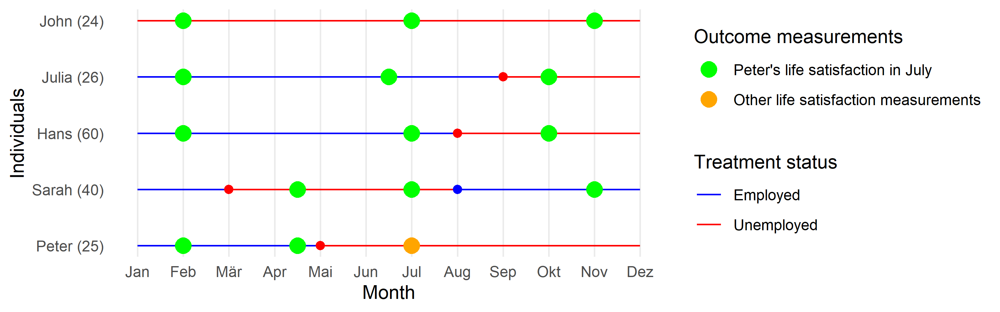
Exercise: Employment and life satisfaction
- We want to estimate the causal effect for Peter: \(\text{Life Satisfaction}_{Peter}(\color{red}{\text{Unemployed}})\) \(- \text{Life Satisfaction}_{Peter}(\color{blue}{\text{Employed}})\) at \(t = July\) (yellow point).
- Q: What is shown on the graph below?
- Q: At \(t = July\), do we observe Peter’s outcome under treatment (unemployed) or under control (employed)?
- Q: Which green measurement point would you pick as a comparison for Peter’s yellow measurement? And why?
ATE: Average Treatment Effect
- Average Treatement Effect (ATE): The average difference in the pair of potential outcomes (averaged over the entire population of interest)
- \(ATE = E[Y_{i}(1) - Y_{i}(0)]\) (time is omitted from the notation)
- Q: Which observations does that concern in the table below?
| \(Unit\) | \(D_{i} (Aspirin:Yes/No)\quad\) | \(Y_{i}(1) (Headache \mid Aspirin)\quad\) | \(Y_{i}(0) (Headache \mid NoAspirin)\) |
|---|---|---|---|
| Simon | 1 | 0 | ? |
| Julia | 1 | 1 | ? |
| Paul | 0 | ? | 1 |
| Trump | 0 | ? | 0 |
| Fabrizio | 0 | ? | 0 |
| Diego | 0 | ? | 0 |
- Again.. can’t estimate ATE without observing both potential outcomes (even with infinite sample size)
Why? moving from ITE to ATE?
- \(ITE\) is unobservable
- Average Treatment Effect (\(ATE\)) = Diff. in averages
- \(ATE\) can be estimated relying on less daring assumptions (Holland 1986, 948f)
- e.g., (proper) random assignment (should) partly satisfy them (“statistical solution”)
- Important: \(ATE = E[Y_{i}(1) - Y_{i}(0)]\): is the expected value of the unit-level treatment effect under the distribution induced by sampling from the super-population (= ATE in super-population) (Imbens and Rubin 2015, 117)
- Estimating Population ATE (PATE) \((ATE_{sp} = \tau_{sp} = \mathbb{E}_{sp})\) from Sample ATE (SATE) \((ATE_{fs} = \tau_{fs})\) requires random sample (Holland 1986, Imai 2008)
- \(_{fs}\) = finite sample, \(_{sp}\) = super population (= target population)
ATE: Naive Estimate
- Naive estimate of ATE: Difference between expected values in treatment and control
- Equate \(E[Y_{i}(1)]\) - \(E[Y_{i}(0)]\) with \(E[Y_{i}|D=1] - E[Y_{i}|D=0]\)
- \(E[Y_{i}|D=1] - E[Y_{i}|D=0] = ({\color{red}{0+1}})/2 - ({\color{orange}{1+0+0+0}})/4 = 0.5 - 0.25 = 0.25\)
| \(Unit\) | \(D_{i} (Aspirin: Yes/No)\quad\) | \(Y_{i} (Headache: Yes/No)\quad\) |
|---|---|---|
| Simon | 1 | 0 |
| Julia | 1 | 1 |
| Paul | 0 | 1 |
| Trump | 0 | 0 |
| Fabrizio | 0 | 0 |
| Diego | 0 | 0 |
- Q: What is the problem with the naive estimate of the treatment effect? Can we interpret 0.25 as causal effect? Why (not)?
ATE: Decomposition
| \(Unit\) | \(D_{i} (Aspirin: Yes/No)\quad\) | \(Y_{i} (Head.: Yes/No)\quad\) | \(Y_{i}(1) (Head. \mid YesAspirin)\quad\) | \(Y_{i}(0) (Head. \mid NoAspirin)\) |
|---|---|---|---|---|
| Simon | 1 | 0 | 0 | ? |
| Julia | 1 | 1 | 1 | ? |
| Paul | 0 | 1 | ? | 1 |
| Trump | 0 | 0 | ? | 0 |
| Fabrizio | 0 | 0 | ? | 0 |
| Diego | 0 | 0 | ? | 0 |
- ATE can be decomposed as a function of 5 quantities (e.g., Keele 2015, 4)
- \(\underbrace{E[Y_{i}(1) - Y_{i}(0)]}_{\substack{ATE}}\) = \({\color{violet}\pi}\) \((\underbrace{E[\color{red} {Y_{i}(1)|D_{i} = 1}] - E[\color{blue}{Y_{i}(0)|D_{i} = 1}]}_{\substack{ATT}})\) + \((1 - {\color{violet}\pi})(\underbrace{E[\color{green}{Y_{i}(1)|D_{i} = 0}] - E[\color{orange}{Y_{i}(0)|D_{i} = 0}]}_{\substack{ATC}})\)
- \({\color{violet}\pi}\): proportion of sample assigned to treatment (2/6 = 0.33..)
- e.g., \(E[\color{red} {Y_{i}(1)|D_{i} = 1}]\): Average pot. outcome under treatment, given units are in treatment condition
- Q: What do the following terms describe? \(E[\color{blue}{Y_{i}(0)|D_{i} = 1}]\); \(E[\color{green}{Y_{i}(1)|D_{i} = 0}]\); \(E[\color{orange}{Y_{i}(0)|D_{i} = 0}]\)
- Q: In your own words, which parts do we have and which parts don’t we have?
ATE: Identification Problem
- Observed (measured)
- \({\color{violet}\pi}\) using \(E[{\color{violet}{D_{i}}}]\)
- \(E[\color{red} {Y_{i}(1)|D_{i} = 1}]\) using \(E[Y_{i}\mid D_{i} = 1]\)
- \(E[\color{orange}{Y_{i}(0)|D_{i} = 0}]\) using \(E[Y_{i}\mid D_{i} = 0]\)
- Unobserved (not measured)
- \(E[\color{blue}{Y_{i}(0)|D_{i} = 1}]\): Average outcome under control \((Y_{i}(0))\), given units in treatment condition \((...|(D_{i}=1))\)
- \(E[\color{green}{Y_{i}(1)|D_{i} = 0}]\): Average outcome under treatment \((Y_{i}(1))\), given units in control condition \((...|(D_{i}=0))\)
- \(E[Y_{i}(1) - Y_{i}(0)]\) = 2/6 \(\times\) (0.5 - ?) + 4/6 \(\times\) (? - 0.25)
| \(Y = 1\) | \(Y = 0\) | |
|---|---|---|
| \(D = 1\) | 0.5 | ? |
| \(D = 0\) | ? | 0.25 |
- Identification Problem!
- Two quantities are unobservable
- Just as for ITE we must rely on assumptions to identify ATE (fill em in)
Causal estimands & notation (1)
Potential outcomes: Sometimes \(Y_{i}(1)\) written as \(Y_{1i}\), \(Y_{i}^{t}\), \(y_{i}^{1}\) (Morgan and Winship 2007, 43)
ATE notation (finite vs. superpopulation, Imbens and Rubin (2015, 18))
- Finite sample: \(ATE_{fs} = \tau_{fs} = \frac{1}{N} \sum_{i=1}^{N} (Y_{i}(1) - Y_{i}(0))\)
- Superpopulation: \(ATE_{sp} = \tau_{sp} = \mathbb{E}_{sp} = E[Y_{i}(1) - Y_{i}(0)] = \mathbb{E}_{sp}[Y_{i}(1) - Y_{i}(0)]\)
Causal estimands & notation (2)
Often the focus is on subpopulations (Imbens and Rubin 2015, 18)
Females (covariate value): \(\tau_{fs} (f) = \frac{1}{N(f)} \sum\limits_{i: X_{i} = f}^{N} (Y_{i}(1) - Y_{i}(0))\) (Conditional ATE)
- e.g., average effect of drug only for females
ATT: \(\tau_{fs,t} = \frac{1}{N_{t}} \sum\limits_{i: D_{i} = 1}^{N} (Y_{i}(1) - Y_{i}(0))\)
- Average effect of the treatment for those who were exposed to it
- Q: How could we write the ATC?
Other subpopulations: Complier Average Treatment Effect; Intent-to-Treat Effect (see overview at Egap)
Causal estimands & notation (3): Exercise
Q: For which units in the Table below would you need to fill in the missing potential outcomes if you were interested in…
- …the average treatment effect: \(\small ATE_{fs} = \tau_{fs} = \frac{1}{N} \sum_{i=1}^{N} (Y_{i}(1) - Y_{i}(0))\)?
- …the average treatment effect on the treated: \(\small ATT_{fs} = \tau_{fs,t} = \frac{1}{N_{t}} \sum\limits_{i: D_{i} = 1}^{N} (Y_{i}(1) - Y_{i}(0))\)?
- …the conditional average treatment effect for males: \(\small ATE_{fs,m} = \tau_{fs} (m) = \frac{1}{N(m)} \sum\limits_{i: X_{i} = m}^{N} (Y_{i}(1) - Y_{i}(0))\)?
- …the conditional average treatment effect on the treated for males: \(\small ATT_{fs}(m) = \tau_{fs, t} (m) = \frac{1}{N_{t}(m)} \sum\limits_{i: D_{i} = 1, X_{i} = m}^{N} (Y_{i}(1) - Y_{i}(0))\)?
| \(Unit\) | \(D_{i}\) | \(Y_{i}(1)\) | \(Y_{i}(0)\) |
|---|---|---|---|
| Simon | 1 | 0 | ? |
| Julia | 1 | 1 | ? |
| Paul | 0 | ? | 1 |
| Trump | 0 | ? | 0 |
| Fabrizio | 0 | ? | 0 |
| Diego | 0 | ? | 0 |
(Key) Assumptions
- Often causal identification concerns defending several key assumptions (e.g., Keele 2015)
Causal ordering assumption: Written as \(D_{i} \longrightarrow Y_{i}\) (Imai’s notation)
- No reverse causality: \(D_{i}\not\longleftarrow Y_{i}\)
- No simultaneity: \(D_{i}\not\longleftrightarrow Y_{i}\)
Independence assumption (IA): also called unconfounded assignment (For other names see Imbens and Rubin 2015, 43)
Stable Unit Treatment Values Assumption (SUTVA): (1) No interference assumption & (2) Consistency assumption
- We’ll talk about 2. and 3. now and other ones later
Assumptions: Independence Assumption (IA)
- IA = Treatment status is independent of potential outcomes \((Y_{i}(1), Y_{i}(0) \perp D_{i})\)
- i.e., assignment status unrelated to potential outcomes…
- …whether you take aspirin or not is independent of what outcome you would have under treatment/control
- Violation: e.g., experimenter knows how patients respond to aspirin and assigns accordingly
- Insight: Under IA “expectation(s) of the unobserved potential outcomes is equal to the conditional expectations of the observed outcomes conditional on treatment assignment” (Keele 2015, 5)
- IA allows us to connect unobservable potential outcomes to observable quantities in the data
- IA is linked to the “assignment mechanism” (see (Imbens and Rubin 2015, 14) for a recent discussion)
- Why does the indpendence assumption (+ SUTVA below) identify causal effect? (next slide)
Assumptions: Independence Assumption (IA)
- Under the IA: ATE = \(\underbrace{E[Y_{i}(1) - Y_{i}(0)]}_{\substack{unobserved}} = E[Y_{i}(1)] - E[Y_{i}(0)] = \underbrace{E[Y_{i}|D_{i} = 1] - E[Y_{i}|D_{i} = 0]}_{\substack{observed}}\)
- We can replaces potential outcomes with observed outcomes
| \(Unit\) | \(D_{i}\quad\) | \(Y_{i}\quad\) | \(Y_{i}(1)\quad\) | \(Y_{i}(0)\) |
|---|---|---|---|---|
| Simon | 1 | 0 | 0 | ? |
| Julia | 1 | 1 | 1 | ? |
| Paul | 0 | 1 | ? | 1 |
| Trump | 0 | 0 | ? | 0 |
| Fabrizio | 0 | 0 | ? | 0 |
| Diego | 0 | 0 | ? | 0 |
- The IA allows us to equate the expected value of the whole column \(E[Y_{i}(1)]\) (red and green values) with the observed red values, i.e. \(E[Y_{i}|D_{i} = 1]\) (same for column \(E[Y_{i}(1)]\)).
- \(E[Y_{i}|D_{i} = 1] \stackrel{1}{=} E[(Y_{i}(0) + D_{i}(Y_{i}(1) - Y_{i}(0))| D_{i} = 1] \stackrel{2}{=} E[Y_{i}(1)|D_{i} = 1] \stackrel{3}{=} E[Y_{i}(1)]\)
- See next slide for explanation of step \(\stackrel{1}{=}\), \(\stackrel{2}{=}\) and \(\stackrel{3}{=}\)
- Same logic for \(E[Y_{i}\mid D_{i} = 0] = E[Y_{i}(0)]\)
Assumptions: Independence Assumption - Steps
Step \(\stackrel{1}{=}\): In causal inference, the observed outcome \(Y_{i}\) can be expressed as a combination of potential outcomes \(Y_{i}(0)\) and \(Y_{i}(1)\) based on the treatment indicator \(D_{i}\) (Observed Outcome Definition). Specifically, \(Y_{i} = Y_{i}(0) + D_{i} (Y_{i}(1) - Y_{i}(0))\).
- This means that if the individual \(i\) does not receive the treatment (\(D_{i} = 0\)), their outcome is \(Y_{i}(0)\). If they do receive the treatment (\(D_{i} = 1\)), their outcome is \(Y_{i}(1)\).
Step \(\stackrel{2}{=}\): If \(D_{i} = 1\), \((Y_{i}(0) + 1\times Y_{i}(1) - 1\times Y_{i}(0))\) so \(Y_{i}(0)\) cancels out and we end up with \(E[Y_{i}(1)\mid D_{i} = 1]\)
Step \(\stackrel{3}{=}\): Because \(Y_{i}(1)\) is independent of \(D_{i}\) (independence assumption) we can replace \(E[Y_{i}(1)\mid D_{i} = 1]\) with \(E[Y_{i}(1)]\)
Longer explanation
- To estimate the ATE we would need to calculate the expected value of the differences between potential outcomes in column \(Y_{i}(1)\) and column \(Y_{i}(0)\). In other words, we would have to observe both treatment and control units in their counterfactual states (e.g., observe what the value of control units would be if they had been treated). However, for the units that were assigned to control \(D_{i} = 0\) we do not observe \(Y_{i}(1)\) and the other way round.
- Starting with the column \(Y_{i}(1)\), the independence assumption simply means that the expected value of the whole column \(E[Y_{i}(1)]\) (red and green values) can be equated with the expected value of the first two rows of the column, namely \(E[Y_{i}(1)\mid D_{i} = 1]\) (the red values). And that is what we actually observe. Hence, through this assumption there is no need to observe the missing green values any more. The same logic applies to column \(Y_{i}(0)\). The IA allows us to equate the expected value of the whole column \(E[Y_{i}(0)]\) (blue and orange values) with the orange values, i.e. \(E[Y_{i}(0)\mid D_{i} = 0]\).
Independence assumption & random assignment
- Q: Imagine the students in our class were randomly split into two groups, a treatment group and a control group. What would be your expectation regarding the distribution of … across the two groups?
- Observable characteristics (Gender, age, skin color)
- Unobservable characteristics (blood pressure, happiness)
- Possible responses to experimental treatment (reaction to aspirin)
- Random assignment
- = a statistical solution (Holland 1986, 948f)
- Units randomly assigned to treatment/control have identical distributions of covariates/potential outcomes in both groups (long run!)
- “if the physical randomization is carried out correctly, then it is plausible that S [= treatment status D] is independent of \(Y_{t}\) [ \(Y_{i}(1)\) ], and \(Y_{c}\) [ \(Y_{i}(0)\) ], and all other variables over U [the super population]. This is the independence assumption.” (Holland 1986, 948).
- Random assignment induces independence between treatment status and potential outcomes
- Random assignment induces independence between treatment status and potential outcomes
- Q: What does in the long run mean?
Assumptions: SUTVA
- SUTVA: Stable Unit Treatment Values Assumption
- -1- No interference & -2- Consistency: No hidden variations of treatment
- The potential outcomes for any unit do not vary with the treatments assigned to other units
- A subject’s potential outcome is not affected by other subjects’ exposure to the treatment
- Imai’s notation: \(Y_{i}(D_{1},D_{2},...,D_{n})=Y_{i}(D_{i})\)
- For each unit, there are no different forms or versions of each treatment level, which lead to different potential outcomes (Imbens and Rubin 2015, 10; Keele 2015, 5)
- Unambiguous definition of exposure, e.g. “15 min of exercise” (Keele 2015, 5)
- No hidden multiple versions/different administration of treatment
- Imai’s notation: \(Y_{i}=Y_{i}(d)\text{ whenever } D_{i}=d\)
Assumptions: SUTVA Exercise (1)
Insight: If we assume SUTVA! (Imbens and Rubin 2015, 10)
- Each individual faces same number of treatment levels (2 in aspirin example)
- Potential outcomes are a function of only our individual actions (e.g., not influenced by others in this room)
Q: Imagine you all have a headache and you sit in the same room. Then we try to randomly assign aspirin to one half of you to test its effect: What would the two assumptions (No interference, No hidden variations) mean and how could they be violated in that situation? Discuss in groups!
Q: In groups, think of one more empirical examples where those assumption could be violated.
Assumptions: SUTVA Exercise (2)
- Q: Below you find examples for planned experiments. Discuss in groups of 2 or 3.
- What is the unit in these examples? How could the independence assumption and the SUTVA assumption be violated when those experiments are implemented?
- Private lessons \((D)\) → School performance \((Y)\)
- In a Mannheim school, half of the 10% worst performing pupils in each class are randomly assigned to receiving private lessons.
- In-person teaching \((D)\) → student satisfaction \((Y)\)
- To test the reception of online-teaching, a unversity decides to randomly assign half of the seminars to in-person teaching, the other half to online teaching.
- Job-training programme \((D)\) → Unemployment \((Y)\)
- Half of Mannheim’s unemployed are randomly assigned to a job training program.
- COVID19 drug \((D)\) → survival \((Y)\)
- 50% of the COVID19 patients at a Mannheim hospital are randomly assigned a new, promising drug in a placebo trial.
Quiz
- See here.
Session 5
Randomized experiments: Ideal, lab, natural and field experiments
Intro
Questions?
Q: What is the fundamental problem of causal inference? (missing data!)
Assumptions example: Campaign Advertisement and Vote Choice (1)
- Research question: What is the effect of a campaign advertisement on an individual’s vote choice (Party A vs. B)?
- Treatment \(D_{i}\): Exposure to the campaign advertisement
- Outcome \(Y_{i}\): Individual’s vote choice.
- Causal Ordering Assumption \(D_{i} \longrightarrow Y_{i}\): implies that treatment causes outcome and not the other way around
- No reverse causality \(D_{i}\not\longleftarrow Y_{i}\): implies that an individual’s vote choice does not influence whether or not they were exposed to the campaign advertisement
- No simultaneity: \(D_{i}\not\longleftrightarrow Y_{i}\): implies that treatment and outcome do not occur simultaneously, i.e., exposure to advertisement \(D\) occurs before the vote choice \(Y\) is made
- Practice: ensure this by timing exposure to advertisement \(D\) before voting choice \(Y\) is made and by randomizing advertisement exposure to avoid selection bias where more likely voters for Party A are more exposed to the advertisement
Assumptions example: Campaign Advertisement and Vote Choice (2)
- Independence Assumption \((Y_{i}(1), Y_{i}(0) \perp D_{i})\): states that treatment assignment is independent of potential outcomes
- i.e., the exposure to the advertisement should not be correlated with other factors that might influence the vote choice which can be achieved through randomization
- Stable Unit Treatment Value Assumption (SUTVA)
- No Interference: treatment of one individual does not affect the outcomes of another individual
- e.g., one person’s exposure to the advertisement does not influence another person’s vote choice
- Consistency Assumption: For each unit, there are no different forms or versions of each treatment level, which lead to different potential outcomes (unambiguous definition of exposure)
- e.g., if an individual is exposed to the advertisement, their vote choice reflects the effect of seeing that specific advertisement which is the same for other treated individuals (analogue for individuals in control)
- SUTVA violated if individuals discuss the advertisement with each other, thereby indirectly affecting each other’s vote choices or if advertisement is different across treated individuals
- No Interference: treatment of one individual does not affect the outcomes of another individual
Ensuring Assumptions in Practice
To ensure these assumptions hold in a real study:
- Randomization: Randomly assign individuals to either the treatment group (exposed to the advertisement) or the control group (not exposed)
- Timing Control: Ensure that the exposure to the advertisement occurs well before the vote choice is made to avoid simultaneity
- Isolation: Conduct the experiment in a way that minimizes interaction between subjects to prevent interference
- Measurement: Carefully measure the vote choice after the exposure period to ensure that the treatment effect is captured accurately.
- Treatment design:: Make sure treatment/control is unambiguously defined across experimental subjects
Experimental vs. observational studies
Distinction going back to Cochran (1965) and others
Assignment mechanism: “process that determines which units receive which treatments, hence which potential outcomes are realized and thus can be observed [and which are missing]” (Imbens and Rubin 2015, 31)
Experiments (experimental studies)
- Assignment mechanism is both known and controlled by the researcher
- Q: What do we mean by “controlled by” and how does assignment in an experiment normally work?
Observational studies
- Assignment mechanism is not known to, or not under the control of, the researcher.
- e.g., with survey data we can NOT decide who gets treated (e.g., education, divorce) and who doesn’t
Field experiments
- A randomized intervention in the real world rather than in artificial, controlled setting of a laboratory
- Examples
- Remedying Education: Evidence from Two Randomized Experiments in India (Banerjee et al. 2007)
- “two randomized experiments conducted in schools in urban India. A remedial education program hired young women to teach students lagging behind in basic literacy and numeracy skills. It increased average test scores of all children in treatment schools by 0.28 standard deviation, mostly due to large gains experienced by children at the bottom of the test-score distribution.”
- The Mark of a Criminal Record (Pager 2003)
- “The present study adopts an experimental audit approach—in which matched pairs of individuals applied for real entry‐level jobs—to formally test the degree to which a criminal record affects subsequent employment opportunities.”
- Causal effect of intergroup contact on exclusionary attitudes (Enos 2014)
- “Here, I report a randomized controlled trial that assigns repeated intergroup contact between members of different ethnic groups. The contact results in exclusionary attitudes toward the outgroup.”
- Durably reducing transphobia: A field experiment on door-to-door canvassing (Broockman2016-oa?)
- “we show that a single approximately 10-minute conversation encouraging actively taking the perspective of others can markedly reduce prejudice for at least 3 months. We illustrate this potential with a door-to-door canvassing intervention in South Florida targeting antitransgender prejudice”
- Remedying Education: Evidence from Two Randomized Experiments in India (Banerjee et al. 2007)
Natural experiments
- Assumption: “a real world situation that produces haphazard [random] assignment to a treatment” (Rosenbaum 2010, 67)
- Examples
- Does indiscriminate violence increase insurgent attacks? (Lyall 2009)
- “This proposition is tested using Russian artillery fire in Chechnya (2000 to 2005) to estimate indiscriminate violence’s effect on subsequent patterns of insurgent attacks across matched pairs of similar shelled and nonshelled villages.”
- The Republicans Should Pray for Rain: Weather, Turnout, and Voting in U.S. Presidential Elections (Gomez 2007)
- Does indiscriminate violence increase insurgent attacks? (Lyall 2009)
- Criticism
- When Natural Experiments Are Neither Natural nor Experiments (Sekhon 2012)
- Design drives questions… researcher roaming around in search of natural experiments
Exercise: Lab vs. field vs. natural experiments
- Q: What do you think are the advantages and disadvantages of lab, field and natural experiments? Discuss in groups.
Ideal Experiments & Ideal Research Designs (IRDs): Exercise
- IRD: “the study a researcher would carry out to answer a research question if there weren’t any practical, ethical or resource-related constraints” (Bauer and Landesvatter 2023)
- Research question: What is the causal effect of victimization on social trust (trust in strangers)? (Bauer 2015)
- Research question: What is the causal effect of fake news about immigrants on vote choice for the AfD? (similarly to Bauer and Clemm von Hohenberg 2021)
- Q: If you had no (practical, ethical, financial) constraints what would your study look like? Develop one with your neighbour(s).
- What is the target population you want to study? (let’s take University Freiburg students)
- What is your sample?
- Where would the experiment take place?
- How would you construct the treatment?
- Which units in the sample get treated? When are the treated or not?
- How would you measure individuals’ vote choice/trust? When would you measure it? etc.
Paper: From ideal experiments to ideal research designs (IDRs) (Bauer and Landesvatter 2023)
- Review how methodologists define and advocate using ideal experiments (IEs) (Section 2)
- (Re-)introduce the concept of an ideal research design (IRD) vs. ARD (Section 3)
- Contrasting IRDs and ARDs: An example (Section 4)
- Departing from our more systematical account of IRDs we review whether and how empirical researchers have used ideal experiments and ideal research designs in applied empirical work (Section 5)
Summary
- Randomized experiments are seen as the “gold standard”
- Researcher controls assignment of units to treatment and control
- Randomization breaks any link between covariates/potential outcomes and the treatment(independence assumption holds!)
- We know the assignment mechanism
- Bernoulli trial (coin flip): In the long run (with many units), treated and control groups will be identical in all respects, observable and unobservable on average
- Other randomization types (e.g., stratified randomization) may yield more precise causal inferences when N limited and/or potential outcomes vary with covariates
- Lab vs. field vs. natural experiments: Pros & cons
- Ideal research designs (experiments) as benchmarks
Session 6
Experiments: Analysis and checks
Retake
- Imbens and Rubin (2015) use \(W\) as letter for treatment not \(D\) (don’t get confused!)
- Q: Why don’t we use \(T\)?
- Naming: Ideally use same name for a concept but usage differs..
- independence assumption (e.g., Keele 2015) = unconfoundedness assumption (Imbens and Rubin 2015)
- Controlling = conditioning; Treatment effect = causal effect
- Ideal experiment example: Bauer (2015)
Randomized experiments: Analysis & checks (1)
Provided perfect randomization we can estimate causal effect by comparing outcome averages between treatment and control group (e.g., using t-tests)
- But different randomization designs may require different stat. approaches (Imbens and Rubin 2015)
Various checks are recommended!
Examples from…
- Enos 2014 (field experiment): Is there a causal effect of Causal effect of intergroup contact on exclusionary attitudes?
- Bauer & Clemm von Hohenberg 2021 (survey experiment): Is there a causal effect of source characteristics (and content) on belief in and sharing of their information? (see appendix for treatment)
Randomized experiments: Analysis & checks (2)
- Various checks are recommended (2-6 also useful for non-experiments):
- (1) Did the randomization really work?
- (2) Are treatment groups really balanced in terms of covariates?
- (3) Did participants really (not) “take” the treatment?
- (4) Is the sample representative of a larger target population?
- (5) Are different participants affected differently by the treatment?
- (6) How long does the treatment effect operate? (treatment lag & decay)
Analysis & checks (1)
- (1) Did the randomization really work?
- Enos (2014): Compare sizes of treatment groups (Q: Where?)
Analysis & checks (2)
- (1) Did the randomization really work?
- Enos (2014): Compare sizes of treatment groups
- Randomization into 6 groups: \(2 \times 2 \times 2\) (Source \(\times\) Channel \(\times\) Content)
- Enos (2014): Compare sizes of treatment groups
Analysis & checks (3)
- (2) Are treatment groups really balanced?
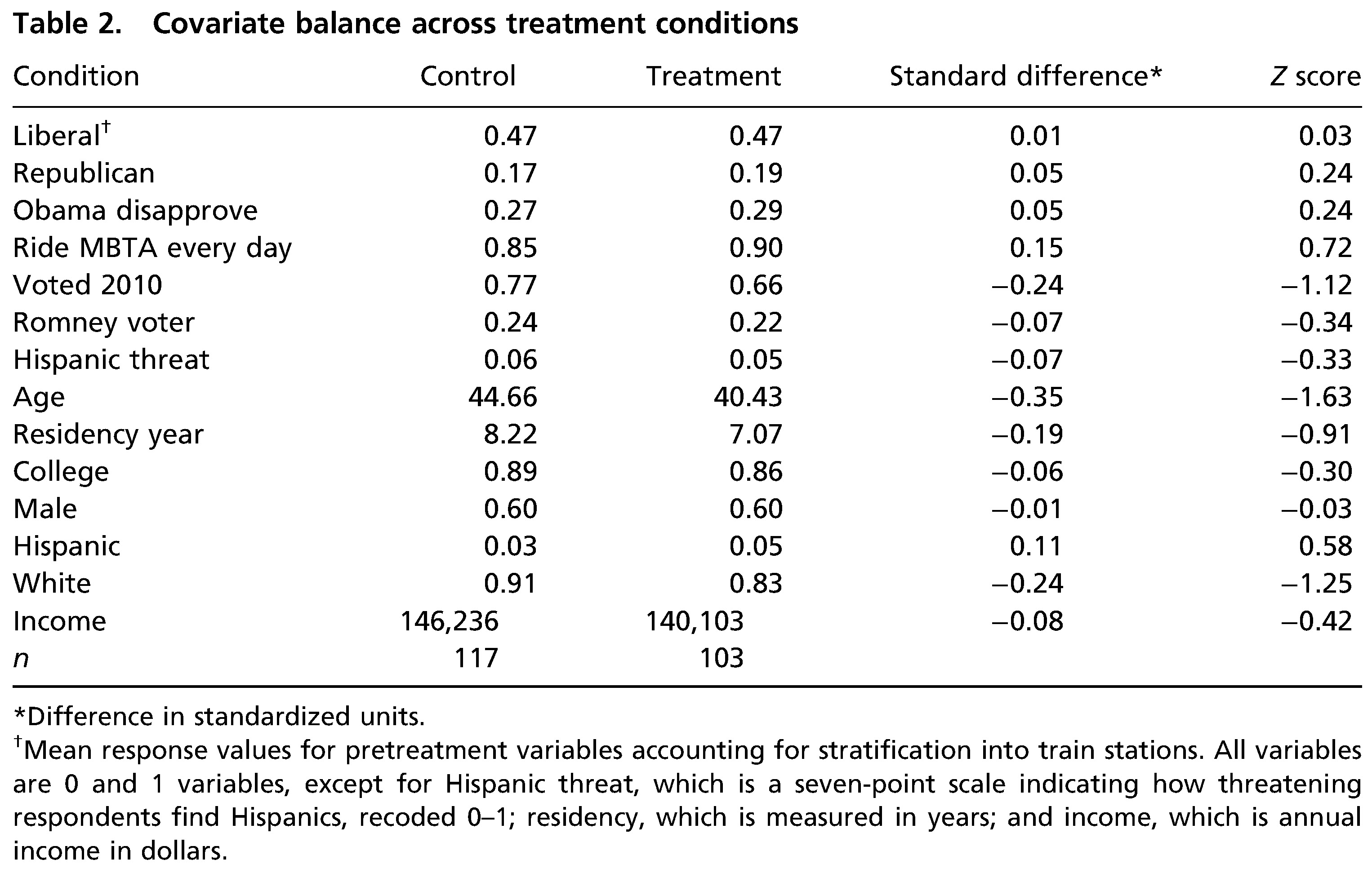
- Bauer and Clemm von Hohenberg (2021): Compare covariate distributions across treatment groups
Analysis & checks (4)
- (2) Are treatment groups really balanced?
- Bauer and Clemm von Hohenberg (2021): Compare covariate distributions across treatment groups
Analysis & checks (5)
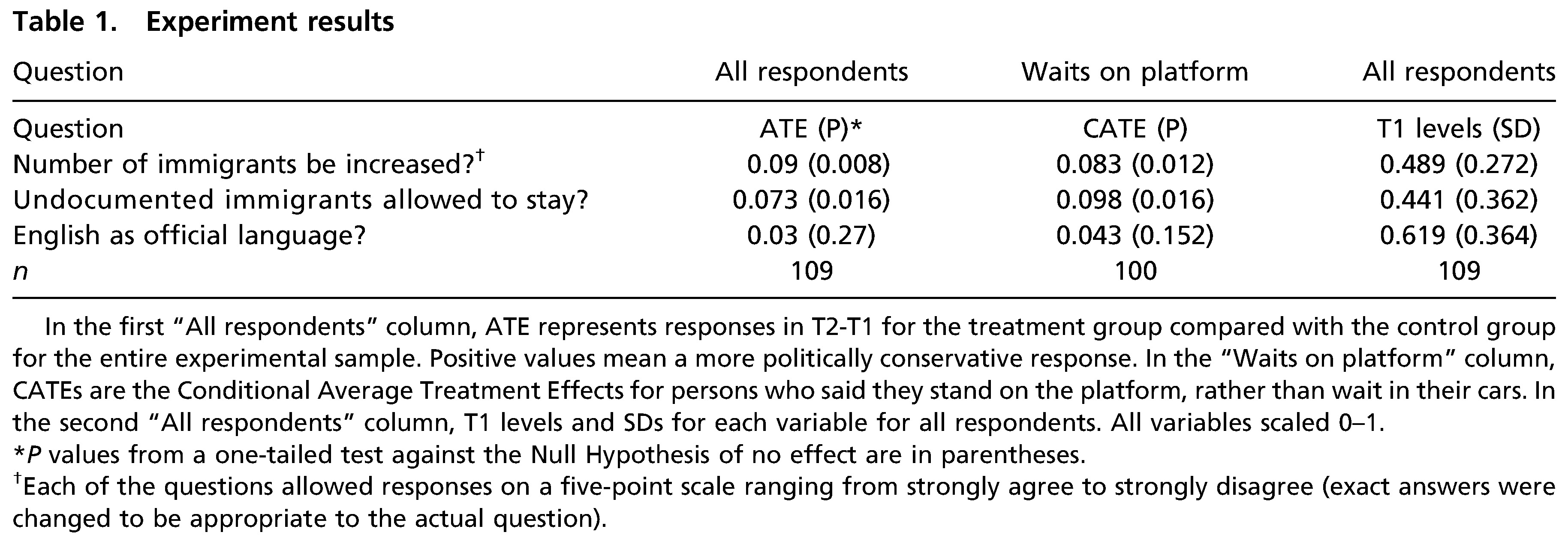
- (3) Did participants really (not) “take” the treatment?
- Enos (2014): Provide analysis for subsets that are more likely to have been exposed (waiting on the platform)
Analysis & checks (6)
- (3) Did participants really (not) “take” the treatment?
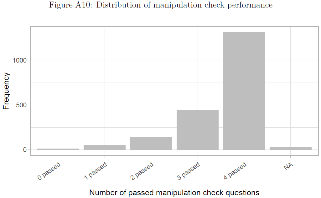
- Bauer and Clemm von Hohenberg (2021): Build in manipulation checks testing whether participants have seen or read the treatment & estimate effects for subsets that passed the checks
Analysis & checks (7)
- (4) Is the sample representative of a larger target population?
- Bauer and Clemm von Hohenberg (2021): Q: How would you proceed? What can we learn from the table below?
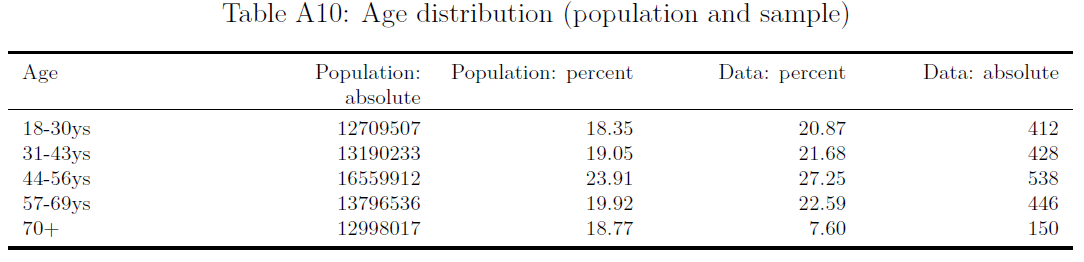
- Enos (2014): e.g., argues that the “Census Tracts used in this experiment had a mean of just 2.8% Hispanic, making the communities tested here both demographically typical and representative of the type of community in which demographic change has not already occurred.” (p. 3700)
Analysis & checks (8)
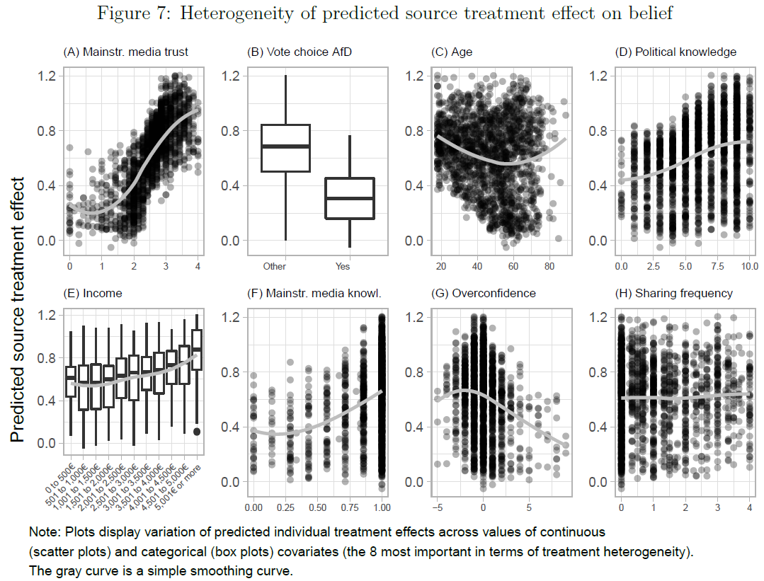
- (5) Are different participants affected differently by the treatment?
- Bauer and Clemm von Hohenberg (2021): Explore treatment heterogeneity through interactions or with ML methods
Analysis & checks (9)
- (6) How long does the treatment effect operate? (treatment lag & decay)
- Enos (2014): Measure the outcome at different time points post-treatment
Analysis & checks (10): More checks
- Attrition (cf. Enos 2014, 3704)
- If outcome measured at two time points make sure to check whether units dropped out for second measurement
- Q: What is a possible disadvantage of measuring the outcome before the treatment?2
- SUTVA violation
- No interference: Try to observe interactions or ask whether they took place or exclude observations where you suspect interference
- Consistency/no hidden variations: Try to observe or ask whether people really got/took the same treatment
- Measurement error
- Pre-test measures, e.g., pre-test survey and ask respondents whether they understood questions
Experimental vs. observational studies
- Q: What was the main difference between experimental (experiments) and observational studies again?
- Experiments (experimental studies)
- Assignment mechanism is both known and controlled by the researcher
- Observational studies
- Assignment mechanism is not known to, or not under the control of, the researcher
We are leaving the realm of experimental studies and enter the realm of observational studies!
Good because.. many questions cannot be answered using experiments! (ethical & resource constraints)
Lab: Experimental data
- You can find the files for the lab in this folder.
- Please download the following files and store them in a directory that you use for this course (this will be your working directory).
Lab_2_Experimental_data.htmlLab_2_Experimental_data.qmdLab2_data
- Please download the following files and store them in a directory that you use for this course (this will be your working directory).
Quiz
- Please do the quiz.
Session 7 & 8
Selection on Observables: Theory
Intro
Questions?
Today’s objective
- Discuss strategies when we don’t have experimental data
- Data: Cross-sectional data, i.e., variables measured once (usually at the same moment in time)
Terminology: Conditioning on vs. controlling for
Experimental vs. observational studies
Assignment mechanism: “process that determines which units receive which treatments, hence which potential outcomes are realized and thus can be observed [and which are missing]” (see Imbens and Rubin 2015, 31)
Q: What is the difference between experimental (experiments) and observational studies?
- Experiments (experimental studies inlcude lab & field experiments)
- Assignment mechanism is both known and controlled by the researcher
- Researcher randomly assigns units to treatment and control
- We know the function of \(Pr(\mathbf{D}|\mathbf{X},\mathbf{Y}(0),\mathbf{Y}(1))\)!
- Observational studies (e.g., Imbens and Rubin 2015, 41)
- Assignment mechanism is not known to, or not under the control of, the researcher
- Researcher can not randomly assign units to treatment and control
- We don’t know the functional form
- We are leaving the realm of experimental studies and enter the realm of observational studies!
Observational studies (1)
Many questions cannot be answered using experiments (Q: Any examples?)
Imbens and Rubin (2015) show that under certain assumptions assignment mechanism within subpopulations of units with the same value for the covariates (Q?) can be interpreted as if it was completely randomized experiment (see Imbens and Rubin 2015, 257)
- Albeit an experiment with unknown assignment probabilities for the units
- Assumptions (see also Imbens and Rubin 2015, 257, 262, 43)
- Unconfounded assignment or uncounfoundedness (= conditional independence): Assignment free from dependence on the potential outcomes
- Probabilistic assignment: Probability of receiving any level of the treatment is strictly between zero and one for all units
- Individualistic assignment: Probability for unit \(i\) is essentially a function of the pre-treatment variables for unit \(i\) only, free of dependence on the values of pre-treatment variables for other units (Q: What is difference to SUTVA?3)
- Assumption (2) & (3) often glossed over (see Imbens and Rubin 2015, 43)
Observational studies (2)
I & R call assignment mechanisms that fulfill those assumptions regular assignment mechanism
Given assumptions 1-3 the probability of receiving the treatment is equal to \(e(x)=N_{t}(x)/(N_{c}(x)+N_{t}(x))\) for all units with \(X_{i}=x\) conditional on the number of treated and control units composing such a subpopulation
- \(N_{t}(x)\) or \(N_{c}(x)\) are the number of units in treatment and control groups with pre-treatment value \(X_{i}=x\)
- \(e(x)\) is also called the Propensity score4
We don’t know a priori assignment probabilities for units, but know that units with the same pre-treatment covariate values have same \(e(x)\), i.e., the same prob. of getting the treatment
This insight still suggests feasible strategies (e.g., focus on subsample)!
Q: What might be the problem if we have many distinct values of covariates?
Exercise 1: Conditioning on covariates (1)
- Q: Which persons would you compare (use) in the table below if you want to condition on gender, i.e., hold the value of the covariate gender constant ( \(X_{i}=1\), \(X_{i}=0\) ) and focus on the respective subsamples (subsetting!)?
| \(Unit\) | \(D_{i}\) | \(X_{i}\) | \(Y_{i}\) | \(Y_{i}(1)\) | \(Y_{i}(0)\) |
|---|---|---|---|---|---|
| Simon | 1 | 0 | 0 | 0 | ? |
| Julia | 1 | 1 | 1 | 1 | ? |
| Paul | 0 | 0 | 1 | ? | 1 |
| Sarah | 0 | 1 | 0 | ? | 0 |
| Fabrizio | 0 | 0 | 0 | ? | 0 |
| Diego | 0 | 0 | 0 | ? | 0 |
Exercise 1: Conditioning on covariates (2)
- Below we colored individuals for which \((\color{#984ea3}{X_{i} = 1})\) and \((\color{#fb9a99}{X_{i} = 0})\).
| $Unit$ | $D_{i}$ | $X_{i}$ | $Y_{i}$ | $Y_{i}(1)$ | $Y_{i}(0)$ |
|---|---|---|---|---|---|
| Simon | 1 | 0 | 0 | 0 | ? |
| Julia | 1 | 1 | 1 | 1 | ? |
| Paul | 0 | 0 | 1 | ? | 1 |
| Sarah | 0 | 1 | 0 | ? | 0 |
| Fabrizio | 0 | 0 | 0 | ? | 0 |
| Diego | 0 | 0 | 0 | ? | 0 |
- Q: Imagine we study the causal effect of education (MA sociology degree: Yes, no) on income (in Euros): Do you think the assumption of unconfoundedness/conditional independence is realistic when we only condition on gender?
Exercise 2: Conditioning on covariates (1)
- Q: On the left you find the joint distribution of outcome Trust (Y), treatment Victimization (D) and covariate Education (X).
- If victimization had been randomly assigned, would estimating the causal effect require conditioning for education (= holding education constant)?
- Which conditional distribution do we focus on if we were to hold Education constant at \(X_{i}=6\)? And \(X_{i}=2\)?
- You assume cond. independence/unconfoundedness for subpopulations of values of the Education variable (i.e., victimization should be as good as random). Within which partitions of the sample would you then compare victims to non-victims?
Exercise 2: Conditioning on covariates (2)
- Conditional distributions are colored in orange: \((\color{orange}{X_{i}=6})\) and \((\color{orange}{X_{i}=2})\).
- Important notion: Condition/control = filtering (Pearl et al. 2016, 8)
- when we condition on X, we filter the data into subsets based on values of X (Pearl et al. 2016, 8) [hold values of X constant]
- Subsequently, we would estimate the treatment effect in those subsets and average it (in some way)
Unconfoundedness/cond. independence assumption
- Why is the unconfoundedness/conditional independence assumption so relevant?
- Most widely used assumption in causal research (Imbens and Rubin 2015, 262)
- Often combined with other assumptions (often implicitly)
- e.g., exogeneity assumption combines unconfoundedness with functional form and constant treatment effect assumptions that are quite strong, and arguably unnecessary
- → here focus on cleaner, functional-form-free unconfoundedness assumption
- Comparison with other assumptions highlights its attractiveness
- Unconfoundedness implies that one should compare units similar in terms of pre-treatment variables (compare “like with like”)
- → has intuitive appeal and underlies many informal/formal causal inferences
- In its absence we would need other additional assumptions that provide guidance on which control units would make good comparisons for particular treated units (and vice versa)
- Q: How should we select covariates for conditioning (controlling/filtering)?
Covariate selection for conditioning & bias
Remember.. fundamental objective: Estimate true causal effect of D on Y without bias (unbiased)
Common-cause confounding bias (Elwert and Winship 2014b, 37)
- D ← X → Y
- results from failure to condition on a common cause (a confounder) of treatment and outcome
Overcontrol/post-treatment bias
- D → X → Y
- results from conditioning on a variable on a causal path between treatment and outcome (Elwert and Winship 2014b, 35–36)
Endogenous selection bias
- D → X ← Y
- Collider variable: A common outcome of D and Y
- results from conditioning on a collider (or its descendant) on a non-causal path linking treatment and outcome
Covariates: confounding/post-treatment bias
- Example: Party identification → Vote choice (U.S. examply by King 2010)
- Q: What covariates should we control for/condition on? Why or why not? And what biases may we introduce/avoid in doing so? (always indicate when X is measured)
- Possible covariates
- race
- education
- gender
- voting intentions measured five minutes before vote choice
- Q: What do we mean by “unbiased” and “bias can go in both directions”? Example?
- Q: Does it matter when the covariates are measured?
- Yes, always consider when covariates are measured (or better ‘happened’), i.e., before, between or after treatment D and outcome Y!
Covariates: endogenous selection bias
- Talent T, Beauty B, Hollywood success S (Elwert and Winship 2014b, 36)
- RQ: Is there a causal effect of Talent T → Beauty B?
- Asume talent and beauty are unrelated (no causal relationship)
- Assume both T and B separately cause success S: T → S ← B
- Hollywood success S is a collider variable (common outcome of T and B)
- Endogenous selection bias if conditioning on/controlling for collider (Elwert and Winship 2014b, 36)
- Given success (S = 1), i.e., conditioning on and looking at subset of successful Hollywood actors
- …knowing that non-talented person (T = 0) is successful actor implies that the person must be beautiful (B = 1)
- …knowing that non-beautiful person (B = 0) is a successful actor implies that the person must be talented (T = 1)
- In subsets of Hollywood success (S = 1 or 0) there is a correlation between T and B
- Conditioning on collider (y) creates spurious association between beauty and talent (spurious association is endogenous selection bias)
- Given success (S = 1), i.e., conditioning on and looking at subset of successful Hollywood actors
Exercise: Covariates & bias
- Q: Discuss in groups: A friend of yours wants to investigate the causal effect of having studied (yes vs. no) at \(t_0\) on individuals’ income 20 years later \(t_1\). Your friend wants to control (condition on) different covariates but is nervous because she heard that one might introduce different biases. She is considering the covariates below. Please indicate whether one should control for the following variables (“Yes” vs. “No”) in this concrete example and what kind of bias they may introduce or avoid.
- Marital status at the age of 35
- Parents’ educational level
- Piano lessons during childhood
- Intelligence test in school
- Work experience at the age of 16
- Job skill-level (low vs. high) in his/her forties
Covariates: Summary
- Choice of covariates for conditioning
- Yes: Covariates that affect both D and Y (confounders)
- No: Covariates the lie on the path between D and Y (post-treatment variables)
- No: Covariates that are affected by D and Y (colliders)
- All empirical papers, top 3 political science journals, 2010-2015
- “40% explicitly conditioned on a post treatment variable […] 27% conditioned on a variable that could plausibly be posttreatment […] 33% […] no post-treatment variables included in their analyses […] two-thirds […] that make causal claims condition on post treatment variables.” (Acharya, Blackwell, and Sen 2015, 1)
- Q: How about other disciplines?
Selection on Observables: Lab
Lab: Observational data
- In practice, we usually use a linear regression model to estimate effect of \(D\) on \(Y\) controlling for/conditioning on all relevant covariates \(Xs\)
- ..we will do this in the lab!
- You can find the files for the lab in this folder.
- Please download the following files and store them in a directory that you use for this course (this will be your working directory).
Lab_3_SSO_Observational_data.htmlLab_3_SSO_Observational_data.qmdLab3_data.csv
- Please download the following files and store them in a directory that you use for this course (this will be your working directory).
Quiz
- Link: See email.
Session 9
Matching: Theory
Intro
- Questions?
- Quick wrap up of previous sessions
- RQs; Research design; Population & sample; Measurement; Data (distributions)
- Potential outcomes framework (def. of causal effect), ITE, Naive est., ATE, Assumptions: independence assumption, SUTVA
- Experimental data: Randomization; Field & natural experiments; Ideal experiments; Analytics & checks of rand. experiments
- Observational data: Observational studies (conditional independence assumption!); Conditioning (+ choice of covariates); Confounder, post-treatment and collider bias
- Today: Cross-sectional observational data & estimation strategies & matching
Strategies for Estimation
Remember: In randomized experiments we can simply compare means in treatment and control
Observational studies (and data) require more refined estimation strategies
4 (+1) broad classes of strategies for estimation (Imbens and Rubin 2015, 268f)
- All four aim at estimating unbiased treatment (causal) effects
- Model-based imputation (1), weighting (2), blocking [i.e., subclassification] (3), and matching methods (4) (+ 5th combines aspects)
Strategies (1) and (2-4) differ in that (2-4) can be implemented before seing any outcome data
- Prevents researcher from adapting the model to fit his/her priors about treatment effect
We focus on model-based imputation (1) (= regression) and matching methods (4)
Model-based imputation (1)
Theory: Impute missing potential outcomes by building a model for the missing outcomes
- Use model to predict what would have happened to a specific unit had this unit been subject to the treatment to which it was not exposed
In practice: “off-the-shelf” methods
- Typically linear models (regression) are postulated for average outcomes, without a full specification of the conditional joint potential outcome distribution (Imbens and Rubin 2015, 272f)
But model-based imputation problematic when covariate distributions are far apart!
Better: Prior to using regression methods ensure balance between covariate distributions for treatment and control
Model-based imputation (2)
- Data: \(\small N_{t}\) =42; \(\small N_{c}\) =150 (subset visualized)
- Education: Mean 2.81 for treated and 5.01 for control units
- Q: Is the covariate distribution of Education (X) across treatment and control balanced?
- LM: \(\small y_{i} = \underbrace{\color{magenta}{\beta_{0}} + \color{orange}{\beta _{1}} \times d_{i} + \color{orange}{\beta _{2}} \times x_{i}}_{\text{Modell} = \color{green}{\widehat{y}}_{i} = \text{Predicted values}} + \underbrace{\color{red}{\varepsilon}_{i}}_{\color{red}{Error}} = \color{green}{\widehat{y}}_{i} + \color{red}{\varepsilon}_{i}\)
- Estimates: \(\small \color{magenta}{\beta_{0}}\) =6.02; \(\small \color{orange}{\beta _{1}}\) = -0.51; \(\small \color{orange}{\beta _{2}}\) = 0.06;
- Q: What do we mean by “extrapolation”?
- Model makes predictions for regions where we don’t have observations (e.g., victims with education 7 or higher)
- Pre-processing data makes sense!
- Prune units without equivalent units in treatment or control to balance data
Matching: Basics
“broadly […] any method that aims to equate (or ”balance”) the distribution of covariates in the treated and control groups” (Stuart 2010, 2)
Goal
- Find one (or more) non-treated unit(s) for every treated unit with similar observable characteristics against whom the effect of the treatment can be assessed
- Treatment and control group as similar as possible except for the treatment status (Covariate balance)
Approach
- Exclude/prune (or down-weight) observations without comparable units in both treatment and control
Q: What tradeoff is there when it comes to pruning units (think of representativeness)?
Matching: Why?
Pure regression approach is increasingly questioned (e.g., Aronow and Samii 2015)
Matching methods (Stuart 2010, 2)
- Complementary to regression adjustment
- Reduce imbalance
- Highlight areas of covariate distribution without sufficient overlap/common support between treatment/control (avoid extrapolation)
- Straightforward diagnostics to assess performance
- Makes you think about selection
Q: If we use matching, do we still need the conditional unconfoundedness/independence assumption?
Matching: Overlap & common support I
- Q: Are there areas in the distribution where we don’t have common support across treatment/control focusing on value combinations of education and age?
- Q: If we increase the number of variables (covariates) on which we match. Does that make it more or less difficult to find matches? Exact vs. inexact matching? What might we do with a variable like age before we match?
Matching: Overlap & common support II
- Common support affects what populations we can learn about (namely the subsample for which we have common support)
- “any method would struggle to assess the causal effect of probation [Bewährung] on offenders who committed a very serious crime (e.g., terrorism) because no one sentenced for that crime would receive probation. A lack of common support arises whenever some subpopulation defined by a confounder (e.g., terrorists) contains no treated units or no untreated units (e.g., those on probation or not).” (Lundberg et al. 2021, 539-540)
- Common support problems leave three options (Lundberg et al. 2021, 539-540)
- Argue that feasible subpopulation (with treated and control observations) is interesting in itself
- Argue that feasible subpopulation is still informative about target population
- Lean on parametric model and extrapolate to what they think would happen in the space beyond common support
Matching: Steps
- Select distance measure
- Exact matching (same covariates values)
- One-dimensional summary measure (e.g. Propensity-score, Mahalanobis)
- Caliper: “One strategy to avoid poor matches is to impose a caliper and only to select a match if it is within the caliper.” (Stuart 2010, 10)
- Describes bandwidth that matches are allowed to have (e.g., accept someone aged between 40 and 44 for someone aged 42)
- Matching method (see Savje et al. 2016, 5, Fig. 1)
- Nearest neighbor matching (1:1 or k:1 nearest neighbor, optimal matching, replacement)
- Subclassification, full matching and weighting
- Assessing balance
- Compare covariate distribution between treatment and control
- In practice: one-dimensional measures (std. difference in means, variance ratio etc)
- Repeat prior steps until balance is good
- Analysis of outcome based on matched sample (e.g., estimate regression)
Matching: Exercise - Matching methods
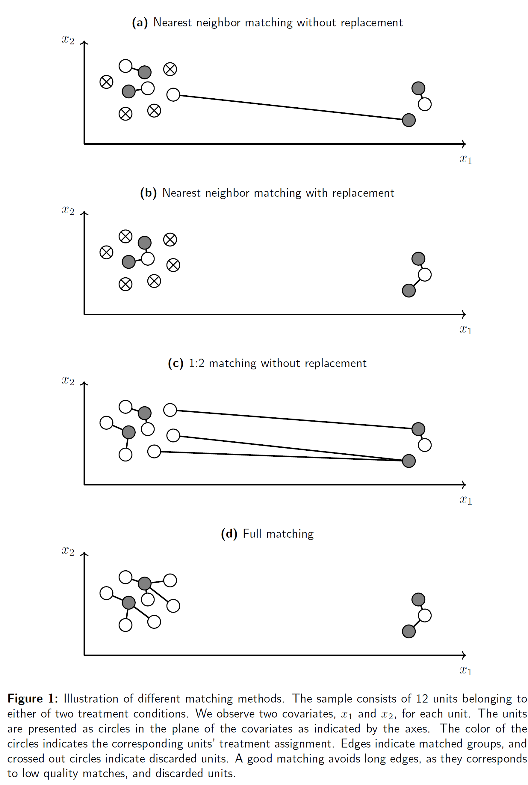
- Q: Discuss the graph (Sävje, Higgins, and Sekhon 2017, fig. 1) in groups (read the description!) and explain what you see in the different panels!
- If the image is too small use right-click to open it in a new window.
- How many dimensions/variables are shown in the graph?
- What are the white/gray/strikethrough circles?
- What are the broad differences between the 4 matching methods? And which one is preferable?
- Explain each panel.
- Does the order in which we find matches matter (why?)?
Matching: Choices
- Distance measures
- In practice: Choose different methods for different variables
- e.g., numeric distance for numeric variables; exact matching for categorical variables
- In practice: Choose different methods for different variables
- Matching methods
- Nearest neighbor matching: “One complication of simple (‘greedy’) nearest neighbormatching is that the order in which the treated subjects are matched may change the quality of the matches. Optimal matching avoids this issue by taking into account the overall set of matches when choosing individual matches, minimizing a global distance measure (Rosenbaum, 2002).” (Stuart 2010, 10)
- Matching with replacement (Stuart 2010, 11)
- Can decrease bias because controls that look similar to many treated individuals can be used multiple times (e.g., in situations where we have few controls)
- Order does not matter (because we can use them multiple times)
- Inference more complex because matched controls no longer independent (e.g. account for that with frequency weights)
- Treatment effect can be based on a very low number of controls
Matching: What to match on?
- Unconfoundedness assumption: Assignment random conditional on covariates
- Match on all observed vars that may affect both treatment D and outcome Y
- Careful: Avoid post-treatment and endogenous selection bias
- Match on quadratic/polynomial terms etc. where it makes sense theoretically (e.g. age X, education D and income Y)
- Ultimate benchmark is balance of covariates X across values of treatment D
- “good balance” depends on your research question and data
- Does it make sense to combine matching with regression (using same covariates)?
- Yes, conceptually you induce independence between Xs and D in the matched sample. But there may still be a direct causal path from Xs on Y, i.e. Xs may explain some of the variation in Y independently from D
- Adding X decreases the amount of unexplained variance in Y, you get more precise estimates (decreases S.E.)
Matching: Assessing balance (Greifer 2021)
Standardized mean differences (SMD): Difference in means of each covariate between treatment/control standardized by a stand. factor (same scale across all COVARs)
- Standardized factor: SD of covariate in treated group (targeting ATT) or pooled SD across both groups (targeting ATE) [+ use same before/after matching]
- SMDs close to zero indicate good balance (Recommended thresholds: .1 and .05) [also compute for squares cubes etc.]
Variance Ratios: Ratio of variance of covariate in one group to that in the other
- Values close to 1 indicate good balance (= similar variances)
Empirical CDF Statistics: Evaluate difference in empirical cumulative density functions (eCDFs) of each covariate between treatment/control (allow assessment of imbalance across the entire covariate distribution)
Visual Diagnostics: Can help tailoring matching method to target imbalance
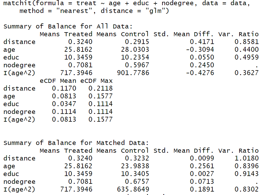
Balancing scores & Propensity score (1)
Idea: find lower-dimensional functions of covariates that suffice for removing bias associated with differences in the pre-treatment variables (Imbens and Rubin 2015, 266f)
- e.g., can we replace our relevant covariates (e.g., education, gender, age) with a balancing score that represents them?
Formally: balancing score is a function of the covariates such that the probability of receiving the active treatment given the covariates is free of dependence on the covariates given the balancing score: \(D_{i} \perp \!\!\! \perp X_{i} | b(X_{i})\)
Important property: if assignment to treatment is unconfounded given the full set of covariates, then assignment is also unconfounded conditioning only on a balancing score
Balancing scores & Propensity score (2)
- Propensity score is a scalar balancing score
- = conditional probability of receiving the treatment given \(X_{i}=x\)
- \(D_{i} \perp \!\!\! \perp X_{i} | e(X_{i})\)
- Estimating the propensity score
- A science in itself… (see Imbens and Rubin 2015, Ch. 13)
- Practice: Estimate a logistic regression in which treatment variable D is predicted by covariates X
- Yields propensity score (probability that someone receives treatment given covariates) as predicted by X
- However we still need to make the unconfoundeness assumption
Matching on propensity score (1)
- Propensity score: Probability of receiving the treatment given the observed covariates
- Propensity score matching developed as part of Rubin causal model
- Estimate logistic regression of covariates on treatment; Predicted values = pr-score
- Example below: We reduce
x_ageandx_education(2 dimensions/variables) topr_score(1 dimension/variable)
| Name | x_education | x_age | d_victim | y_trust | pr_score |
|---|---|---|---|---|---|
| Alissa | 4 | 75 | 0 | 8 | 0.14 |
| Damaris | 0 | 17 | 1 | 7 | 0.50 |
| Juan | 0 | 18 | 0 | 9 | 0.50 |
| Rosa | 6 | 62 | 0 | 5 | 0.11 |
| Janeth | 4 | 62 | 0 | 6 | 0.17 |
| Yeimi | 2 | 51 | 1 | 9 | 0.28 |
| Jacob | 4 | 31 | 0 | 5 | 0.24 |
| Monica | 4 | 38 | 1 | 8 | 0.22 |
| Cesar | 6 | 44 | 1 | 3 | 0.14 |
| Marcos | 0 | 18 | 1 | 5 | 0.50 |
Matching on propensity score (2)
- Criticized by (LaLonde1986-zk?), defended by (Dehejia1999-sp?) and critisized by (King2019-kn?):
- Presentation in the ‘international’ methods colloquium: “We show that propensity score matching (PSM), an enormously popular method of preprocessing data for causal inference, often accomplishes the opposite of its intended goal – increasing imbalance, inefficiency, model dependence, and bias.”5
- Newer developments
- Nonparametric matching methods, e.g., Genetic Matching (Diamond 2013)
- Generalized Full Matching (Sävje, Higgins, and Sekhon 2021)
- “no existing matching method can accommodate the six treatment arms and the 6,762,701 observations involved in the study”
Session 10
Matching: Lab
Lab: Matching
- You can find the files for the lab in this folder.
- Please download the following files and store them in a directory that you use for this course (this will be your working directory).
Lab_4_SSO_Matching.htmlLab_4_SSO_Matching.qmdLab4_data.csv
- Please download the following files and store them in a directory that you use for this course (this will be your working directory).
Session 11
Difference-in-differences - Theory & Lab
Intro
- Questions?
- Today: Observational data & estimation strategies & difference in differences
- Quotes
- “Those who worship at the altar of complex methods are prone to the error of thinking that technical sophistication can substitute for knowledge of the subject matter, careful theorizing, and appropriate research design” (Firebaugh 2008: 207f)
- “We cannot rely on statistical wizardry to overcome faulty data and research design” (Firebaugh 2008: 208)
- Lecture 7 partly material draws on Denis Cohen’s material (co-author on our book)
Reminder: Classical experiment
- The “Classical” Experiment
- Randomly split units into two groups
- Expose one to the treatment but not the other (control group)
- After randomization independence holds: \(Y_{i}(0), Y_{i}(1), X_{i} \perp D_{i}\text{ for all i = 1, ..., N}\)
- Difference-in-Means: \(\hat{\tau} = E[Y_{i}(1)|D_{i} = 1] - E[Y_{i}(0)|D_{i} = 0]\)…
…as an unbiased estimate of the… - …Average treatment effect: \(E[\hat{\tau}] = E[Y_{i}(1)] - E[Y_{i}(0)]\)
- Randomized experiments considered “gold standard” but often not feasible…
Reminder: Observational cross-sectional data
- Outcome Y, covariates X, treatment D measured at one moment in time
- Treatment D is not randomized
- Assumption to identify causal effect (among others)
- Unconfoundedness conditional on covariates (conditional independence)
- Assumption to identify causal effect (among others)
- Carefully choose covariates on which we condition (control for/match on)!
- Confounders but not post-treatment variables/colliders
- Data over time/repeated observations: Sometimes we observe treatment, outcome and covariates at several time points
- e.g., outcomes for the same unit before/after treatment was administered
- In such situations we can exploit other assumptions for causal inference
Data over time
Panel data: Observing units (individuals, countries etc.) several times (Q: Balanced panel?)
- Normally, stored in wide- or longformat
Term time-series data used for countries/country-level measures across time (“aggregated units”)
Identifcation strategies (e.g., Keele 2015, 10)
- Differences-in-differences (DiD)
- Fixed effects (FE), First differences (FD), PanelMatch
Classical FE/FD approaches recently reassessed from causal inference perspective (e.g., Imai & Kim 2019)
Data perspective: Time just another dimension in the joint distribution (see next slides)
Data over time: Joint distribution
- Underlying any statistical model is a joint distribution (remember!)
- Below a 3D joint distribution of a treatment variable (victim D), an outcome (trust Y) and time
- Q: What would be a cross-section in the Figure below?
Wide format vs. long format data
- Wideformat: Individuals/units in rows, Repeated observations across time/variables in columns
| unit | trust.2006 | trust.2007 | Victimization.2006 | Victimization.2007 |
|---|---|---|---|---|
| Peter | 1 | 1 | 0 | 1 |
| Julia | 5 | 5 | 0 | 1 |
| Pedro | 6 | 6 | 1 | 0 |
- Longformat: Observations of same units are stacked on top of each other
| unit | time | trust | Victimization |
|---|---|---|---|
| Julia | 2006 | 5 | 0 |
| Julia | 2007 | 5 | 1 |
| Pedro | 2006 | 6 | 1 |
| Pedro | 2007 | 6 | 0 |
| Peter | 2006 | 1 | 0 |
| Peter | 2007 | 1 | 1 |
DiD Example: Card & Krueger 1994
- Minimum wages and employment: A case study of the fast food industry in New Jersey and Pennsylvania (Card and Krueger 1994)
- “On April 1, 1992, New Jersey’s minimum wage rose from $4.25 to $5.05 per hour. To evaluate the impact of the law we surveyed 410 fast-food restaurants in New Jersey and eastern Pennsylvania before and after the rise. Comparisons of employment growth at stores in New Jersey and Pennsylvania (where the minimum wage was constant) provide simple estimates of the effect of the higher minimum wage. We also compare employment changes at stores in New Jersey that were initially paying high wages (above $5) to the changes at lower-wage stores. We find no indication that the rise in the minimum wage reduced employment.”
- Units = fast-food restaurants; D = minimum wage (0 = same, 1 = increase); Y = (full-time) employment
- Card & Krueger reply (2000): Figure 1 on the right (dark gray = additional counties)
DiD Setup (1)
Two groups of units (e.g., restaurants, individuals)
Outcome Y: Observed twice, before and after treatment (2 timepoints/periods \(t_{0}\) and \(t_{1}\))
Treatment D: happens between \(t_{0}\) and \(t_{1}\)
- Treatment status at \(t_{0}\) and \(t_{1}\) is known (= 0 for all at \(t_{0}\))
Covariates X: Observed at \(t_{0}\) or before
Graph (left) shows average outcome (across time and groups)
Naive strategies:
- \(\scriptsize E[Y_{i}|D_{i} = 1; T_{i} = 1]\) \(\scriptsize- E[Y_{i}|D_{i} = 1; T_{i} = 0]\)
- \(\scriptsize E[Y_{i}|D_{i} = 1; T_{i} = 1]\) \(\scriptsize- E[Y_{i}|D_{i} = 0; T_{i} = 1]\)
- Q: What would this be in the graph on the left?
Problem: Bias due to pre-existing trends/pre-existing differences (Q: ?)
Solution/Idea: Take trend of control group as counterfactual for unobserved trend in treatment group
DiD Setup (2)
- We absorb unit-specific pre-treatment levels in Y through differencing within units
- \(E[Y_{i}(d)|D_{i} = d; T_{i} = 1] - E[Y_{i}(d)|D_{i} = d; T_{i} = 0]\text{ for }d \in {0,1}\)
- i.e., difference between averages of individual changes between \(t_{0}\) and \(t_{1}\) both for treatment and control units (only change is left over)
- Q: Where would we find those averages in the graph on the preceeding slide?
- We absorb pre-existing trends by differencing within-differences across units
- \(\underbrace{E[Y_{i}(1)|D_{i} = 1; T_{i} = 1] - E[Y_{i}(1)|D_{i} = 1; T_{i} = 0]}_{\text{Trend in treatment group}}\) - \(\{\underbrace{E[Y_{i}(0)|D_{i} = 0; T_{i} = 1] - E[Y_{i}(0)|D_{i} = 0; T_{i} = 0]}_{\text{Trend in control group}}\}\)
- Table 1 provides a short example where \(\Delta Y\) reflects differencing within units. Subsequently, we would calculate \((-20 + (- 30))/2 - (-10 + 0)/2 = -15\) (differencing within-differences).
| \(Unit\) | \(D_{i}\) | \(Y_{i, t = 0}\) | \(Y_{i, t = 1}\) | \(\Delta Y\) |
|---|---|---|---|---|
| Restaurant 1 | 1 | 40 | 20 | -20 |
| Restaurant 2 | 1 | 60 | 30 | -30 |
| Restaurant 3 | 0 | 50 | 40 | -10 |
| Restaurant 4 | 0 | 30 | 30 | 0 |
DiD: Assumptions (1)
- What we want to know:
- \(\underbrace{E[Y_{i}(1)|D_{i} = 1; T_{i} = 1] - E[Y_{i}(1)|D_{i} = 1; T_{i} = 0]}_{\text{Trend under treatment for treated units}}\) - \(\{\underbrace{E[Y_{i}(0)|D_{i} = 1; T_{i} = 1] - E[Y_{i}(0)|D_{i} = 1; T_{i} = 0]}_{\text{Trend under control for treated units}}\}\)
- What we do know:
- \(\underbrace{E[Y_{i}(1)|D_{i} = 1; T_{i} = 1] - E[Y_{i}(1)|D_{i} = 1; T_{i} = 0]}_{\text{Trend in treatment group}}\) - \(\{\underbrace{E[Y_{i}(0)|D_{i} = 0; T_{i} = 1] - E[Y_{i}(0)|D_{i} = 0; T_{i} = 0]}_{\text{Trend in control group}}\}\)
- Q: So which assumption do we make here?
- Q: How do we know that the trend in the control group adequately captures the counterfactual trend in the treatment group in absence of the treatment?
DiD: Assumptions (2)
- Parallel trends assumption
- In absence of treatment, the average outcomes for treated and control groups would have followed parallel paths over time (would have seen the same trend/change)
- Put differently
- The counterfactual trend of Y in the treatment group under control would have been the same as that of the actual control group (see next)
- When choosing DiD as identification strategy it’s all about defending the parallel trends assumption
- i.e., argue for similarity between treatment and control group
DiD: Assumptions (3)
- 2D view of the parallel trends assumption (Angrist and Pischke 2008, Fig 5.2.1)
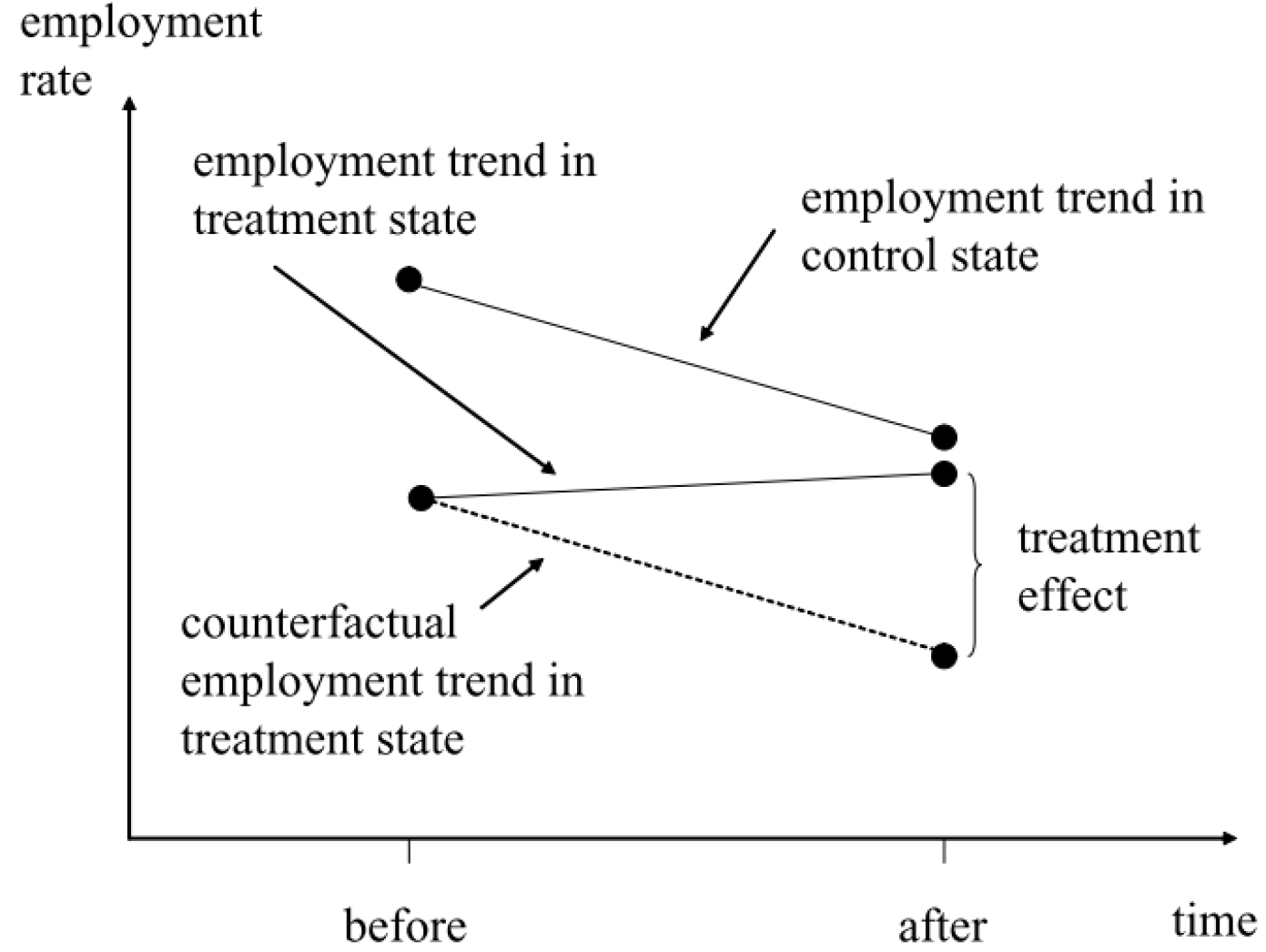
DiD: Causal Identification
- Causal identification in DiD involves:
- Choosing treatment and control groups such that the parallel trend assumptions is plausible
- Employing empirical tests to scrutinize the plausibility of this assumption
- Possible strategies:
- Experimental DiD: Randomization of treatment
- Choose control group that resembles the treatment group as much as possible
- Synthesize control group (e.g., Abadie, Diamond, and Hainmueller 2010)
- Validity checks (see “DiD: Threats to validity”)
DiD: Regression estimation (1)
We can easily estimate our DiD effect via regression.. but how?
We want to estimate:
- \(\hat{\tau} = \underbrace{E[Y_{i}(1)|D_{i} = 1; T_{i} = 1]}_{\text{Treatment group; posttreatment}} - \underbrace{E[Y_{i}(1)|D_{i} = 1; T_{i} = 0]}_{\text{Treatment group; pretreatment}} -\) \(\{\underbrace{E[Y_{i}(0)|D_{i} = 0; T_{i} = 1]}_{\text{Controlgroup; posttreatment}} - \underbrace{E[Y_{i}(0)|D_{i} = 0; T_{i} = 0}_{\text{Controlgroup; pretreatment}}]\}\)
So what do we need?
- a pre-/post-period indicator, \(T_{i} \in \{0,1\}\) (time variable)
- a treatment/control group indicator, \(D_{i} \in \{0,1\}\) (treatment variable)
- an interaction of the two to capture the four combinations of \(D_{i}\) and \(T_{i}\)
DiD: Regression estimation (2)
| name | time T | treated D | outcome Y |
|---|---|---|---|
| Restaurant_1 | 0 | 1 | 15.00 |
| Restaurant_3 | 0 | 1 | 24.00 |
| Restaurant_5 | 0 | 1 | 15.00 |
| Restaurant_2 | 0 | 0 | 40.50 |
| Restaurant_4 | 0 | 0 | 13.75 |
| Restaurant_6 | 0 | 0 | 8.50 |
| Restaurant_1 | 1 | 1 | 27.00 |
| Restaurant_3 | 1 | 1 | 23.00 |
| Restaurant_5 | 1 | 1 | 21.50 |
| Restaurant_2 | 1 | 0 | 24.00 |
| Restaurant_4 | 1 | 0 | 11.50 |
| Restaurant_6 | 1 | 0 | 10.50 |
| time T | treated D | mean_Y |
|---|---|---|
| 0 | 0 | 20.92 |
| 0 | 1 | 18.00 |
| 1 | 0 | 15.33 |
| 1 | 1 | 23.83 |
- Q: Try to write down the DID estimator in potential outcomes notation (previous slide!).
- The DID estimator can be implemented through the following linear model:
- \(\text{outcome Y}_{i} =\) \(\beta_{1} + \beta_{2}\text{time T}_{i} + \beta_{3}\text{treated D}_{i} +\) \(\beta_{4}\text{time T}_{i}\times \text{treated D}_{i}+ \epsilon_{i}\)
- Q: Please explain…
- …how we get from Table 1 to Table 2.
- …to which rows (mean_Y) in Table 2 the terms in the DiD estimator (previous slide) correspond.
- …how (combinations of) the terms in the model (above) may yield estimates of each of the four components (mean_Y values in Table 2).
DiD: Regression estimation (3)
| Dependent variable: | |
outcome Y
|
|
treated D
|
-2.92 |
| (8.02) | |
time T
|
-5.58 |
| (8.02) | |
I(treated D * time T)
|
11.42 |
| (11.35) | |
| Constant | 20.92*** |
| (5.67) | |
| Observations | 12 |
| R2 | 0.14 |
| Adjusted R2 | -0.19 |
| Residual Std. Error | 9.83 (df = 8) |
| F Statistic | 0.42 (df = 3; 8) |
| Note: | p<0.1; p<0.05; p<0.01 |
Equation: \(\text{outcome Y}_{i} =\) \(\beta_{1} + \beta_{2}\text{time T}_{i} + \beta_{3}\text{treated D}_{i} +\) \(\beta_{4}\text{time T}_{i}\times \text{treated D}_{i}+ \epsilon_{i}\)
We can estimate the model for the data above as follows (see left):
- Below we calculate the coefficicents from our group \(\times\) time averages
- \(\beta_{1}\) = 20.92
- \(\beta_{2}\) = 15.33 - 20.92 = -5.59
- \(\beta_{3}\) = 18.00 - 20.92 = -2.92
- \(\beta_{4}\) = Difference between trends = (23.83 - 18.00) - (15.33 - 20.92) = 11.42 (our causal estimate!)
DiD: Regression estimation (4)
- Alternatively, we could difference the outcome beforehand
- Outcome is now \(y_{i,t1} - y_{i,t0}\)
| name | D | Y (T = 0) | Y (T = 1) | Y_diff |
|---|---|---|---|---|
| Restaurant_1 | 1 | 15.00 | 27.0 | 12.00 |
| Restaurant_2 | 0 | 40.50 | 24.0 | -16.50 |
| Restaurant_3 | 1 | 24.00 | 23.0 | -1.00 |
| Restaurant_4 | 0 | 13.75 | 11.5 | -2.25 |
| Restaurant_5 | 1 | 15.00 | 21.5 | 6.50 |
| Restaurant_6 | 0 | 8.50 | 10.5 | 2.00 |
- Estimation with wide-format data
- \(y_{i,t1} - y_{i,t0} = \beta_{0} + \beta _{1} D_{i} + \beta X_{i} + \varepsilon_{i}\)
- Summing up: The kind of model we estimate in R depends on the data structure
- Long-format:
lm(Y ~ D + T + D*T + X, data= data_long) - Wide-format:
lm(Y_diff ~ D + X, data= data_long) - …where
Xare covariates that we can add to make the parallel trends assumption more realistic
- Long-format:
DiD: Threats to validity
- Non-parallel trends (policy literature)
- Policy/Treatment may assign units to treatment and control based on pre-existing differences in outcomes
- Policy/Treatment may assign units to treatment and control according to whom seems most promising to profit from treatment
- Ashenfelter’s dip – participants change behavior in anticipation of policy/treatment
- Restaurants reduce employment because they anticipate increase in minimum wage
- Unemployed people reduce search efforts because they anticipate participation in a measure
- Additonal checks
- If possible, check pre-and post-trends for longer time periods
- Consider alternative control groups
- Estimate effect for placebo outcomes
- Placebo tests of pre-treatment trends (many periods)
Covariates & aggregate units & standard error
- Condition on covariates
- Account for possibility that samples have systematically different characteristics (and would not display parallel trends)
- Choose covariates that were measured at \(t_{0}\) or before
- DiD can be used with individuals and aggregate units (e.g., cities)
- Be aware that composition of aggregate units may change (drop-outs?)
- Sometimes necessary to adjust standard errors as not to understate uncertainty (e.g., if there is geographic closeness)
Session 12a
Regression discontinuity design (RDD)
- See Appendix A: Regression Discontinuity Design: Theory & Lab for longer version.
Basics (1)
Classic and first use: Evaluation of scholarship programs (Thistlethwaite 1960)
All units receive a score (e.g., a grade), and a treatment (e.g., a scholarship) is assigned to those units whose score is above a known cutoff and withheld from those units whose score is below the cutoff
- Score (variable), cutoff and treatment define a RD design
Q: How have you been selected for your BA program?
Features of (all) RDDs
- Conditional probability of actually receiving treatment given the score changes discontinuously at the cutoff (Cattaneo et al. 2019, 9) [see Fig. 1]
- Unlike other non-experimental designs, assignment of treatment follows a rule that is known (at least to the researcher) and empirically verifiable (Cattaneo et al. 2019, 8)
Basics (2)
\(X_{i}\): Score with \(c\) as a known cutoff
- also called running variable, forcing variable or index
\(Z_{i}\) = Assignment variable; \(1 \text{ if } X_{i} \geq c, 0\text{ otherwise}\)
\(D_{i}\): Treatment actually received
Q: Can you give an example of \(X_{i}\), \(Z_{i}\) and \(D_{i}\) for a concrete person, e.g., thinking of access to a Bachelor program?
- We observe outcome under control condition for units below cutoff and outcome under treatment condition for units above cutoff
Basics (3): Sharp vs. Fuzzy RDD
- Important: Assignment to treatment \(Z_{i}\) (e.g., being offered scholarship) not necessarily \(=\) receiving (complying with) treatment \(D_{i}\) (e.g., taking the scholarship)
- Sharp RD: \(Z_{i} = D_{i}\), all units comply with treatment condition they have been assigned to
- Fuzzy RD: \(Z_{i} \neq D_{i}\), some units fail to receive treatment despite having a score above cutoff (and vice versa)
- Q: Explain sharp and fuzzy RD in the case of a Bachelor program were cutoff is a certain grade (1.4)?
Basics (4)
- Observed average outcome given the score & potential outcomes
\[\mathbb{E}[Y_{i}|X_{i}] = \begin{cases} \mathbb{E}[Y_{i}(0)|X_{i}] & \quad \text{if } X_{i} < c\\ \mathbb{E}[Y_{i}(1)|X_{i}] & \quad \text{if } X_{i} \geq c \end{cases}\]
- Sharp RD design exhibits extreme case of lack of common support on \(X\)
- Units in the control and treatment groups cannot have the same value of score \(X\)
- This highlights that RD analysis fundamentally relies on extrapolation towards cutoff point \(c\)
- Central goal of empirical RD analysis
- Adequately perform (local) extrapolation in order to compare control and treatment units
- Basic assumption of comparability
- Units with very similar values of the score but on opposite sides of the cutoff are comparable
Basics (5)
Fund. problem of causal inference: Only observe the outcome under control, \(Y_{i}(0)\), for those units whose score is below the cutoff \(c\), and the outcome under treatment, \(Y_{i}(1)\), for those units whose score is above the cutoff \(c\)
Fig. 3 plots the average potential outcomes given the score, \(E[Y_{i}(1)|X_{i} = x]\) and \(E[Y_{i}(0)|X_{i} = x]\), against the score
We can estimate the regression function \(E[Y_{i}(1)|X_{i}]\) for values of the score to the right of the cutoff because we observe \(Y_{i}(1)\), for every \(i\) when \(X \geq c\) (solid red line)
- And \(E[Y_{i}(0)|X_{i}]\) for values left to the cutoff (solid blue line)
Sharp RD treatment effect: \(\tau_{SRD} = \mathbb{E}[Y_{i}(1) - Y_{i}(0)|X_{i} = c]\)
- Conceptually: what would be the average outcome change for units with score level \(X_{i} = c\) if we switched their status from control to treated?
Example: Meyersson (2014) (1)
- Meyersson (2014): Islamic Rule and the Empowerment of the Poor and Pious
- Research question: What is the impact of having a mayor from an Islamic party on women’s rights (educational attainment of young women)?
- \(\text{Units }i\): Municipalities
- \(Y_{i}\): educational attainment of women, measured as the percentage of women aged 15 to 20 in 2000 who had completed high school by 2000
- \(X_{i}\): vote margin obtained by the Islamic party in the 1994 Turkish mayoral elections, measured as the vote percentage obtained by the Islamic party minus the vote percentage obtained by its strongest secular party opponent
- \(D_{i}\) ( \(T\) in the paper): electoral victory of the Islamic party in 1994, equal to 1 if the Islamic party won the mayoral election and 0 otherwise \((D_{i} = Z_{i})\)
- Methodological challenge: Municipalities where support for Islamic parties is high enough to result in the election of an Islamic mayor (of one of two islamic parties) may differ systematically from municipalities where this is not the case (secular mayor)
- e.g., religiosity (conservative) is a confounder that may affect both treatment (islamic mayor) and outcome (educational attainment of women)
Example: Meyersson (2014) (2)
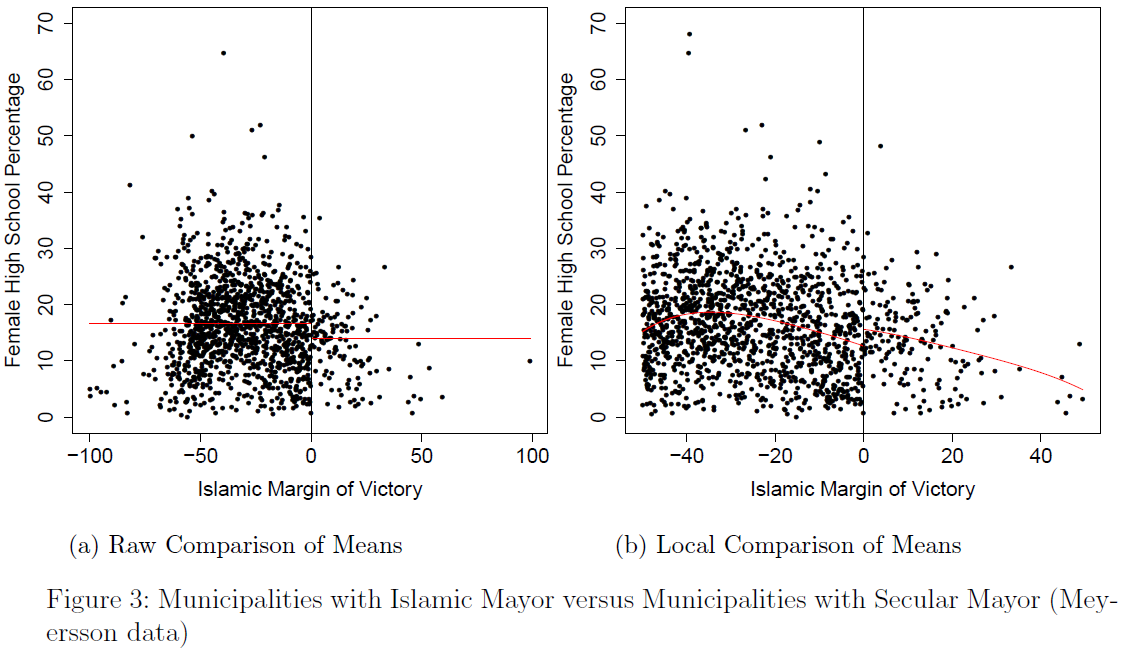
Example: Meyersson (2014) (3)
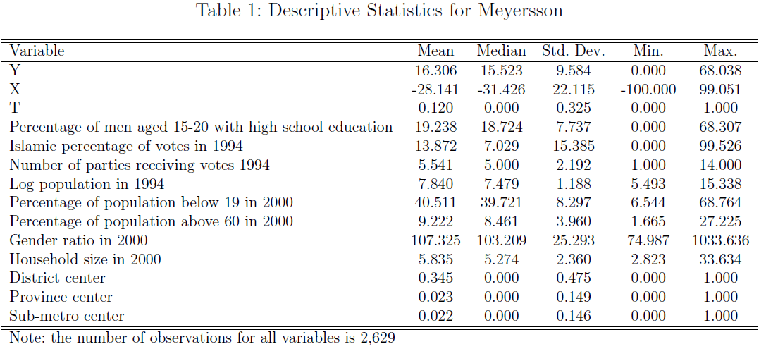
Session 12b
Instrumental variables (IV)
Appendix A: Regression Discontinuity Design: Theory & Lab
Basics (1)
Classic and first use: Evaluation of scholarship programs (Thistlethwaite 1960)
All units receive a score (e.g., a grade), and a treatment (e.g., a scholarship) is assigned to those units whose score is above a known cutoff and withheld from those units whose score is below the cutoff
- Score (variable), cutoff and treatment define a RD design
Q: How have you been selected for your BA program?
Features of (all) RDDs
- Conditional probability of actually receiving treatment given the score changes discontinuously at the cutoff (Cattaneo et al. 2019, 9) [see Fig. 1]
- Unlike other non-experimental designs, assignment of treatment follows a rule that is known (at least to the researcher) and empirically verifiable (Cattaneo et al. 2019, 8)
Basics (2)
\(X_{i}\): Score with \(c\) as a known cutoff
- also called running variable, forcing variable or index
\(Z_{i}\) = Assignment variable; \(1 \text{ if } X_{i} \geq c, 0\text{ otherwise}\)
\(D_{i}\): Treatment actually received
Q: Can you give an example of \(X_{i}\), \(Z_{i}\) and \(D_{i}\) for a concrete person, e.g., thinking of access to a Bachelor program?
- We observe outcome under control condition for units below cutoff and outcome under treatment condition for units above cutoff
Basics (3): Sharp vs. Fuzzy RDD
- Important: Assignment to treatment \(Z_{i}\) (e.g., being offered scholarship) not necessarily \(=\) receiving (complying with) treatment \(D_{i}\) (e.g., taking the scholarship)
- Sharp RD: \(Z_{i} = D_{i}\), all units comply with treatment condition they have been assigned to
- Fuzzy RD: \(Z_{i} \neq D_{i}\), some units fail to receive treatment despite having a score above cutoff (and vice versa)
- Q: Explain sharp and fuzzy RD in the case of a Bachelor program were cutoff is a certain grade (1.4)?
Basics (4)
- Observed average outcome given the score & potential outcomes
\[\mathbb{E}[Y_{i}|X_{i}] = \begin{cases} \mathbb{E}[Y_{i}(0)|X_{i}] & \quad \text{if } X_{i} < c\\ \mathbb{E}[Y_{i}(1)|X_{i}] & \quad \text{if } X_{i} \geq c \end{cases}\]
- Sharp RD design exhibits extreme case of lack of common support on \(X\)
- Units in the control and treatment groups cannot have the same value of score \(X\)
- This highlights that RD analysis fundamentally relies on extrapolation towards cutoff point \(c\)
- Central goal of empirical RD analysis
- Adequately perform (local) extrapolation in order to compare control and treatment units
- Basic assumption of comparability
- Units with very similar values of the score but on opposite sides of the cutoff are comparable
Basics (5)
Fund. problem of causal inference: Only observe the outcome under control, \(Y_{i}(0)\), for those units whose score is below the cutoff \(c\), and the outcome under treatment, \(Y_{i}(1)\), for those units whose score is above the cutoff \(c\)
Fig. 3 plots the average potential outcomes given the score, \(E[Y_{i}(1)|X_{i} = x]\) and \(E[Y_{i}(0)|X_{i} = x]\), against the score
We can estimate the regression function \(E[Y_{i}(1)|X_{i}]\) for values of the score to the right of the cutoff because we observe \(Y_{i}(1)\), for every \(i\) when \(X \geq c\) (solid red line)
- And \(E[Y_{i}(0)|X_{i}]\) for values left to the cutoff (solid blue line)
Sharp RD treatment effect: \(\tau_{SRD} = \mathbb{E}[Y_{i}(1) - Y_{i}(0)|X_{i} = c]\)
- Conceptually: what would be the average outcome change for units with score level \(X_{i} = c\) if we switched their status from control to treated?
Example: Meyersson (2014) (1)
- Meyersson (2014): Islamic Rule and the Empowerment of the Poor and Pious
- Research question: What is the impact of having a mayor from an Islamic party on women’s rights (educational attainment of young women)?
- \(\text{Units }i\): Municipalities
- \(Y_{i}\): educational attainment of women, measured as the percentage of women aged 15 to 20 in 2000 who had completed high school by 2000
- \(X_{i}\): vote margin obtained by the Islamic party in the 1994 Turkish mayoral elections, measured as the vote percentage obtained by the Islamic party minus the vote percentage obtained by its strongest secular party opponent
- \(D_{i}\) ( \(T\) in the paper): electoral victory of the Islamic party in 1994, equal to 1 if the Islamic party won the mayoral election and 0 otherwise \((D_{i} = Z_{i})\)
- Methodological challenge: Municipalities where support for Islamic parties is high enough to result in the election of an Islamic mayor (of one of two islamic parties) may differ systematically from municipalities where this is not the case (secular mayor)
- e.g., religiosity (conservative) is a confounder that may affect both treatment (islamic mayor) and outcome (educational attainment of women)
Example: Meyersson (2014) (2)
Example: Meyersson (2014) (3)
More examples
- Dell, Melissa, and Pablo Querubin. “Nation building through foreign intervention: Evidence from discontinuities in military strategies.” The Quarterly Journal of Economics 133.2 (2018): 701-764.
Local nature of RD effects (1)
- Sharp RD parameter = captures average difference in potential outcomes under treatment versus control
- This average difference is calculated at a single point \((c)\) on the support of a continuous random variable (the score \(X_{i}\))
- Captures a causal effect that is local in nature in contrast to other causal parameters in the potential outcomes framework
- RD treatment effect has limited external validity
- is (often) not representative of treatment effects that would occur for units with scores away from the cutoff
- Meyersson example: Lack of external validity reflected in the focus on close and not all elections
- Figure 3(a) [next slide]: Educational attainment of women seems higher in municipalities where Islamic party looses
- Figure 3(b) [next slide]: Close to \(c\) educ. attainment seems higher in municipalities where Islamic barely wins (zoom in + fourth-orderpolynomial fit)
- By definition: sample of municipalities near the cutoff comprises subset of constituencies where Islamic party is very competitive (localness!)
- …raises the question of how representative they are of wider sample
Local nature of RD effects (2)
Local nature of RD effects (3): Scenarios
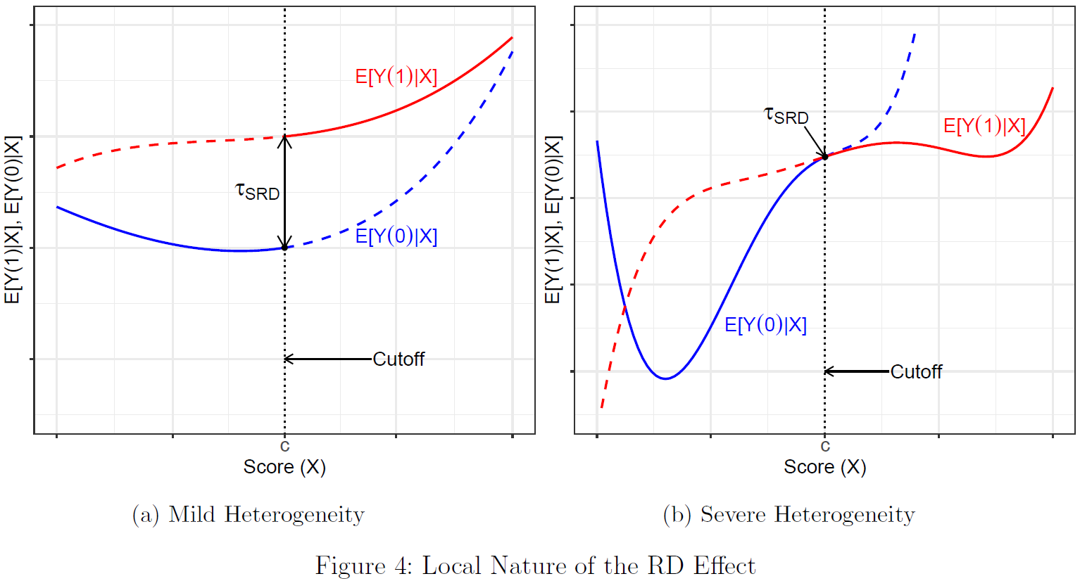
- Q: What do the two scenarios shown in Fig. 4 illustrate (effect sign, e.g., MA program -> income!)? (Cattaneo et al. 2019, 18)
- Increasing external validity of RD estimates is a topic of active research!
Estimation: Continuity-Based Approach (1)
Two approaches to estimation: randomization-based vs. continuity-based approach (we focus on the latter!)
Assumption of comparability formalized by Hahn et al. (2001) using continuity assumptions
- \[\mathbb{E}[Y_{i}(1) - Y_{i}(0)|X_{i} = c] = \lim_{x\downarrow c} \mathbb{E}[Y_{i}|X_{i} = x] - \lim_{x\uparrow c} \mathbb{E}[Y_{i}|X_{i} = x]\]
- They show (in words): If the average potential outcomes are continuous functions of the score at \(c\) (cf. Fig. 4, previous slide), the difference between the limits of the treated and control average observed outcomes – as the score converges to the cutoff – is equal to the average treatment effect at the cutoff
Continuity: As score \(x\) gets closer to cutoff \(c\), the average potential outcome function \(\mathbb{E}[Y_{i}(0)|X_{i} = x]\) gets closer to its value at the cutoff \(\mathbb{E}[Y_{i}(0)|X_{i} = c]\) (same for \(\mathbb{E}[Y_{i}(1)|X_{i} = x]\))
- “key RD identifying assumption is the continuity (or lack of abrupt changes) of the regression functions for treatment and control units at the cutoff in the absence of the treatment” (Cattaneo et al. 2019, 100)
- Continuity: Formal justification for estimating Sharp RD effect by focusing on small neighborhood around cutoff \(c\)
In contrast, randomization-based approach explicitly assumes that RDD induces randomized experiment in window near the cutoff (local randomization assumption)
Estimation: Continuity-Based Approach (2)
- Local polynomial point estimation: Estimate regression functions within bandwith \(h\) around score \(c\)
- This estimation approach is nonparametric because it does not assume a particular parametric form of the regression functions (we just fit a curve to the data)
- Challenge: the unknown regression functions \(\mathbb{E}[Y_{i}(0)|X_{i}=x]\) and \(\mathbb{E}[Y_{i}(1)|X_{i}=x]\) have to be approximated by a polynomial function of the score
- Local polynomial methods implement linear regression fits using only observations near the cutoff point, separately for control and treatment units
- We localize polynomial fit to the cutoff (discarding observations sufficiently far away) and usually employ a low-order polynomial approximation (usually linear or quadratic)
- We only use observations between \(c − h\) and \(c + h\), where \(h > 0\) is so-called bandwidth, i.e., \(h\) determines size of neighborhood around cutoff
- We commonly adopt weighting scheme within bandwidth to ensure observations closer to \(c\) receive more weight (weights determined by a kernel function \(K(·)\))
- Statistical properties of local polynomial estimation and inference depend crucially on the accuracy of the approximation near the cutoff (bandwidth matters!)
Steps: Local Polynomial Point Estimation
Choose a polynomial order \(p\) and a kernel function \(K(\cdot)\).
- \(K(\cdot)\) assigns weights to each transformed observation \((K(\frac{X_{i}−c}{h}))\)
- Choice of \(p\) is more consequential \((p\) = 0 has undesirable properties; higher \(p\) improves accuracy of approximation but increases variabiltiy of estimator + danger of overfitting; preference for local linear RD with \(p=1)\)
Choose a bandwidth \(h\) around \(c\) (see Fig 14, Cattaneo et al. 2019, 46).
For observations above the cutoff, fit a weighted least squares regression of the outcome \(Y_{i}\) on a constant and \((X_{i}−c),(X_{i}−c)^{2},...,(X_{i}−c)^{p}\), where \(p\) is the chosen polynomial order, with weight \(K(\frac{X_{i}−c}{h})\) for each observation. The estimated intercept from this local weighted regression, \(\hat{\mu}_{+}\), is an estimate of the point \(\mu_{+}=\mathbb{E}[Y_{i}(1)|X_{i}=c]\).
- Similar for observations below the cutoff (cf. see Cattaneo et al. 2019, 42 also for equation)
Calculate the Sharp RD point estimate: \(\hat{\tau}_{SRD} = \hat{\mu}_{+} − \hat{\mu}_{-}\)
- Graphically illustrated in Figure 12 on the next slide.
Estimation: Local Polynomial Point Estimation
- Example Figure 12
- Polynomial of order one \((p = 1)\) is fit within bandwidth \(h_{1}\)
- Observations outside \(h_{1}\) are not used
- RD effect is \(\tau_{SRD}=\mu_{+} − \mu_{-}\) and local polynomial estimator of this effect is \(\hat{\tau}_{SRD} = \hat{\mu}_{+} − \hat{\mu}_{-}\)
- Important: Graph shows binned observations!
- Polynomial of order one \((p = 1)\) is fit within bandwidth \(h_{1}\)
- Implementation requires choice of three main ingredients (Cattaneo et al. 2019, 43-51, Fig. 13/14)
- The kernel function \(K(·)\), the order of the polynomial \(p\), and the bandwidth \(h\)
- Using local linear estimation with bandwidth \(h\) and uniform kernel is equivalent to estimating simple linear regression without weights for observations within \(h\)
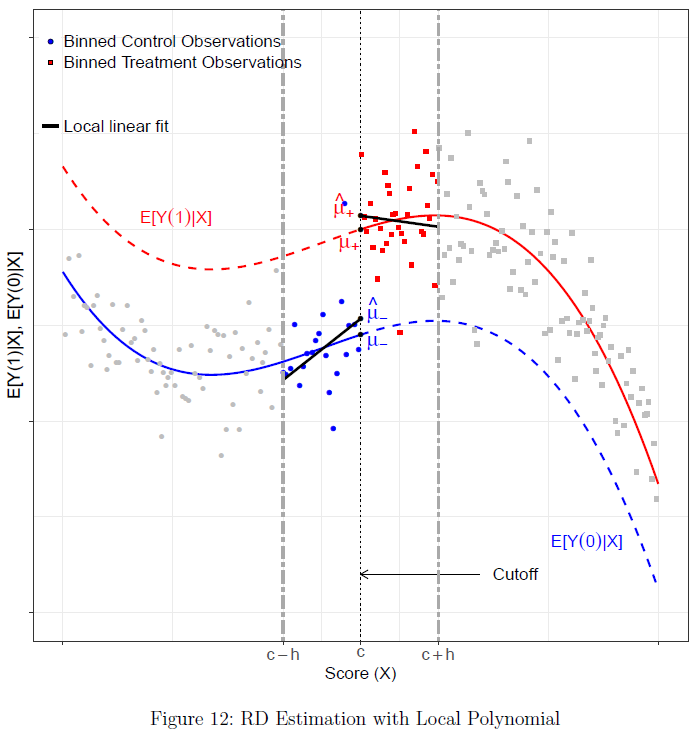
Validation and falsification of RDD
Continuity (and local randomization) assumptions inherently untestable but “empirical implications” testable
General problem: Researcher has no control over assignment
- If cut-off known to units → danger of score change/manipulate
- Q: Can you think of an example of score manipulation?
Qualitative tests of assumptions: Explore how manipulable score/assignment are, e.g., institutional appeal possibility (get scholarship despite low score) or administrative process of score assignment
Quantitative tests of assumptions
- Are treated units near the cutoff similar to control units? Estimate treatment effect on pre-treatment covariates and placebo outcomes (should not be affected!)
- Local N below/above cutoff very different? Explore density of the running variable around the cutoff
- Is estimated difference really due to treatment? Estimate treatment effect at alternative fake/placebo cutoff values
- Sensitivity to observations near the cutoff (4) and bandwith choice (5)
Test: Similarity around the cutoff (1)
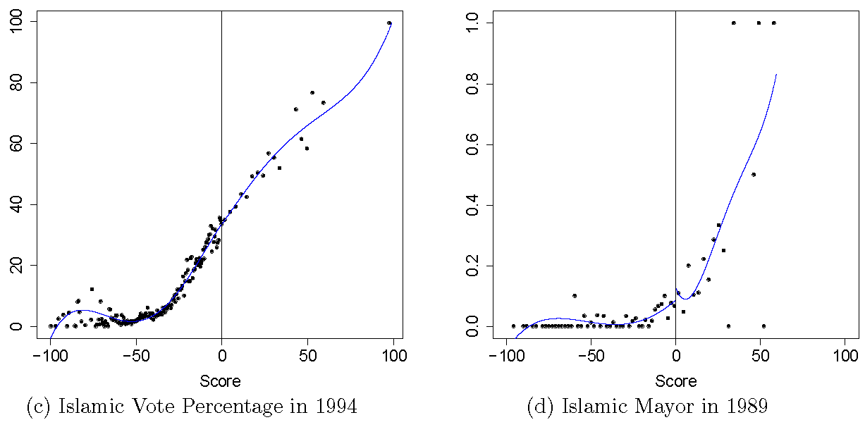
- Estimate treatment effect on pre-treatment covariates and placebo outcomes (Cattaneo et al. 2019, 91, Fig. 16)
- Q: When would the data fail this test, what is the case here and what could it mean substantively?
Test: Density around the cutoff (2)
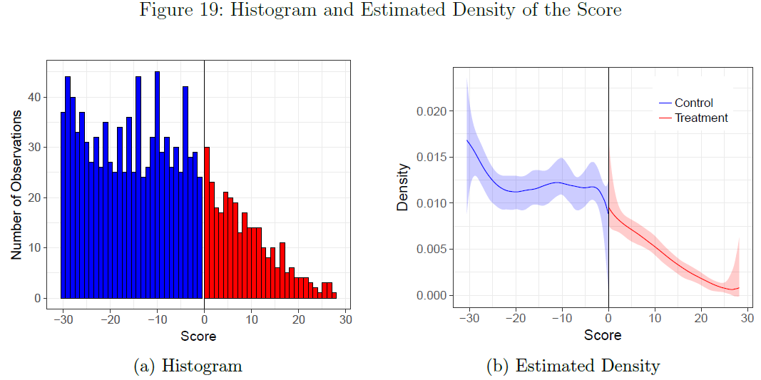
- Visualize density and use hypotheses tests to explore density (= N) around cutoff (Cattaneo et al. 2019, 100, Fig. 19)
- Q: When would the data fail this test and what could it mean substantively?
Test: Placebo cutoffs (3)
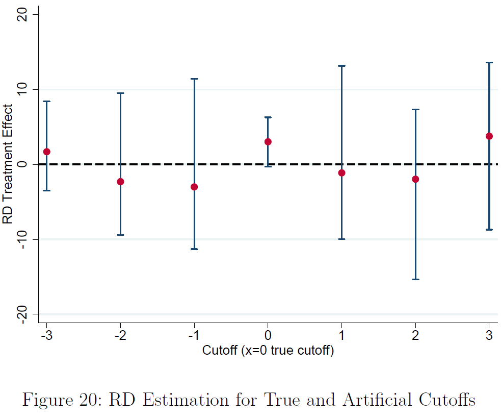
- Key RD identifying assumption continuity (or lack of abrupt changes) at the cutoff in the absence of treatment
- Test whether regression functions for control and treatment units are continuous at points other than the cutoff \(c\)
- Discontinuities away from the cutoff would cast doubt on the RDD
- Q: When would the data fail this test and what could it mean substantively? (Cattaneo et al. 2019, 103, Fig. 20)
Further examples
- Do Harsher Prison Conditions Reduce Recidivism? (Chen and Shapiro 2007)
- Treatment \(D\): Prison conditions
- Outcome \(Y\): Recidivism rates
- Score \(X\): “Upon entry to the federal prison system, an inmate is processed […] individual’s security custody score. The score is intended to predict prisoner misconduct and therefore to measure the supervision needs of individuals.” (Chen and Shapiro 2007, 5)
- Cutoff \(c\): Particular security custody score
- Racial Profiling and Use of Force in Police Stops: How Local Events Trigger Periods of Increased Discrimination (Legewie 2016)
- “I argue that racial bias in the use of force increases after relevant events such as the shooting of a police officer by a black suspect. To examine this argument, I design a quasi experiment using data from 3.9 million time and geocoded pedestrian stops in New York City. The findings show that two fatal shootings of police officers by black suspects increased the use of police force against blacks substantially in the days after the shootings.”
- Treatment \(D\): Fatal shooting of police officer by black suspect
- Outcome \(Y\): Racial bias in the use of force
- Score \(X\): Time
- Cutoff \(c\): Time of the shooting (particular point in time)
- Criticism & warnings: Gelman & Imbens (2019); Review of political science research by Stommes, Aronow, Sävje, 2021
Appendix B: Causal inference with Panel Data
Intro
- Next two sessions: Learning objectives
- …how panel data is structured.
- …panel-data equivalent of cross-sectional potential outcomes.
- …what comparisons we can make using panel data namely within- and between-unit comparisons.
- …common estimators used for panel data (WFE, PanelMatch) and underlying assumptions.
- …the pitfalls of causal panel data analysis, e.g., a potential lack of variation over-time.
- …the most recent statistical software to estimate causal effects with panel data.
Repetition: Cross-sections data, covariates & bias
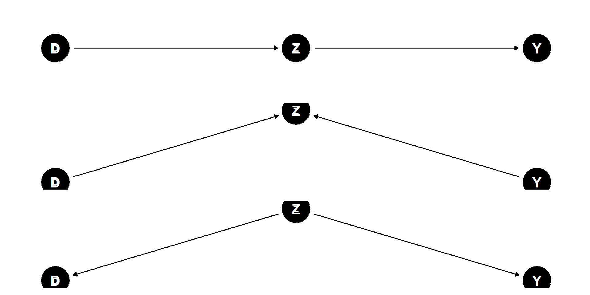
- Q: Which graph on the left corresponds to which of the three biases we discussed? How is Z in the respective situation called? In which of the three situations should we control for Z (or not)?
Repetition: Examples of bias
“If we want to estimate the ATE of social class (D) on educational attainment (Y) and assume D –> educational aspiration (X) –> Y, controlling for aspirations induces ########## bias”
“Education (D) –> SES (Y). We can have a ########## bias if we forget to include parents’ SES (X) because it affects both the education (D) and the SES (Y) of their children.”
“An example of ########## bias would be to control the moisture content of a plant (X) after watering (D), if we are interested in the causal effect of watering plants on growth (Y).”
If interest is causal mediators (i.e., which post-treatment variables matter) → causal mediation analysis
Panel data
Q: Difference-in-differences design/data: How often do we observe (or measure) outcome and treatment?
- Q: What was the main identification assumption? (And for experimental data/cross-sectional data?)
Panel data
- Outcome Y: …is observed twice or more (2+ timepoints)
- Treatment D: …is observed twice or more (2+ timepoints)
- Covariates X: …are observed twice or more (2+ timepoints)
Allows us to focus on changes between time points
Commonly used estimators
- First-difference (FD) estimator & Fixed-effects (FE) estimator
Data structure: Wide format
Data structure: Long format
Potential outcomes in panel data
- Q: How would we define the contemporaneous individual treatment effect (ITE), e.g., for \(\text{Individual}_{i=1, t=2004}\)? And non-contemporeneous, e.g., 3 years later (what about 2?)? How can we calulate/estimate it?
Useful graphs: Treatment variation
- Q: What does the graph show and why is it probably helpful?
Useful graphs: Treatment and outcome trajectory
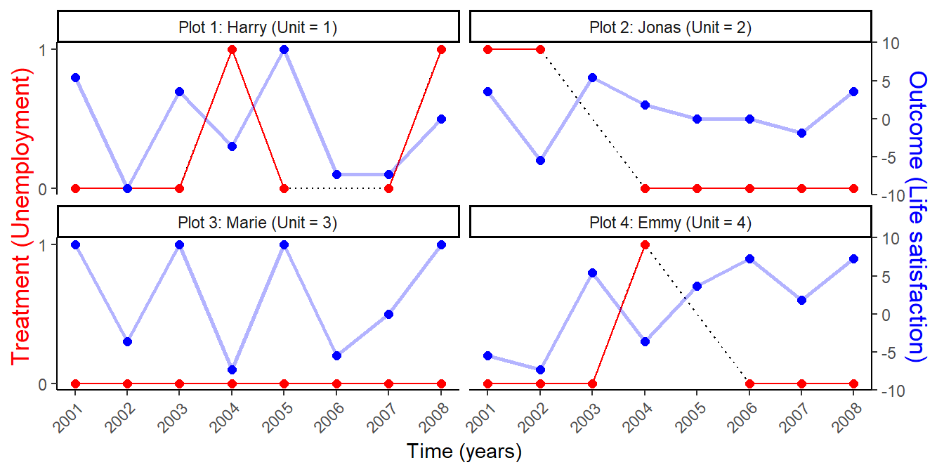
- Q: What does the graph show and why is it probably helpful?
Useful graphs: Variables across time
- Q: What does the graph show and why is it probably helpful?
Two comparative strategies: Within- vs. between-unit
- Q: Does the graph show within- or between-unit comparisons?
First-difference (FD) estimator
- First-difference (FD) estimator (see e.g. Gangl 2010, 33-35)
- \(\Delta y_{it} = y_{it} - y_{it-1} = \theta \Delta d_{it} + \beta \Delta x_{it} + \Delta \varepsilon_{it}\)
- \(i\) is the index for individuals, \(t\) is the index for the time points \((t_{0}, t_{1},t_{2}\text{, etc.})\)
- \(\Delta y_{it}\) is the differenced outcome variable (between \(t_{0}\) and \(t_{1}\) etc.)
- \(\theta\) is the treatment variable coefficient (estimate of the “causal” effect)
- \(\Delta d_{it}\) is the differenced treatment variable \(d\)
- \(\beta \Delta x_{it}\) one differenced covariate \(\Delta x_{it}\) and its effect/coefficient \(\beta\)
- …with more covariates we would have a matrix \(\Delta X_{it}\) of differenced covariates and a vector of \(\beta\)s
- \(\Delta \varepsilon_{it}\) is the differenced error term
- Constant covariates drop out through differencing (cf. top two equations here)
- e.g., if \(\Delta x_{it}\) is constant, difference is 0 and \(\beta \Delta x_{it}\) is 0
- \(\Delta y_{it} = y_{it} - y_{it-1} = \theta \Delta d_{it} + \beta \Delta x_{it} + \Delta \varepsilon_{it}\)
Fixed-effects (FE) estimator
- Fixed-effects (FE) estimator (see e.g. Gangl 2010, 33-35)
- \(y_{it}-{\overline {y_{i}}} = \theta \left(d_{it} - {\overline {d_{i}}}\right) + \beta \left(x_{it} - {\overline {x_{i}}}\right) + \left(\varepsilon_{it} - {\overline {\varepsilon_{i}}}\right)\)
- \(i\) is the index for individuals, \(t\) is the index for the time points \((t_{0}, t_{1}, t_{2}\) etc.)
- \(y_{it}-{\overline {y_{i}}}\) is the de-meaned outcome variable \((\overline {y_{i}}\) = individual mean across time)
- \(\theta \left(d_{it} - {\overline {d_{i}}}\right)\) is the de-meaned treatment variable \(\left(d_{it} - {\overline {d_{i}}}\right)\) and its coefficient \(\theta\) (estimated “causal effect”)
- \(\beta \left(x_{it} - {\overline {x_{i}}}\right)\) is one de-meaned covariate \(\left(x_{it} - {\overline {x_{i}}}\right)\) and its effect \(\beta\)
- …with more covariates we have a matrix of de-meaned covariates and a vector of \(\beta\)s
- \(\left(\varepsilon_{it} - {\overline {\varepsilon_{i}}}\right)\) is a de-meaned error term
- …sometimes error terms for unobserved constant variables are added to the equation to show that they drop out (e.g., see example here).
- Q: What happens to covariates that are constant across time?
- \(y_{it}-{\overline {y_{i}}} = \theta \left(d_{it} - {\overline {d_{i}}}\right) + \beta \left(x_{it} - {\overline {x_{i}}}\right) + \left(\varepsilon_{it} - {\overline {\varepsilon_{i}}}\right)\)
Understanding first-differences and de-meaning
- Q: How would you calculate the \(\Delta y_{it}\), \(\Delta d_{it}\) (first differences), \(y_{it}-{\overline {y_{i}}}\) and \(d_{it} - {\overline {d_{i}}}\) (de-meaned) for Brittany’s trust in the Table below? (same logic for covariates!)
| Name | victim.2006 | victim.2007 | victim.2008 | trust.2006 | trust.2007 | trust.2008 |
|---|---|---|---|---|---|---|
| Brittany | 0 | 0 | 1 | 4 | 4 | 2 |
| Ethan | 1 | 1 | 0 | 5 | 6 | 4 |
| Kyle | 0 | 0 | 0 | 0 | 7 | 5 |
| Jacob | 0 | 1 | 1 | 5 | 3 | 6 |
| Jessica | 0 | 0 | 0 | 7 | 9 | 4 |
- Q: What are the theoretically possible min. and max. values of the differenced outcome variable Y (0-10) and treatment variable D (0,1)?
- Q: What happens to variables that are stable over time? (Think of the difference!)
- Q: What are we comparing here between treatment and control as opposed to cross-sectional data (Hint: Change)?
- Q: What should we control for here since stable covariates drop out of the equation?
- Q: If we look at change for both treatment & outcome between \(t_{0}\) and \(t_{1}\), what additional assumptions are we making (Hint: Temporal order)?
First-differenced and de-meaned data
- Data is simply the differences (change scores) between time points (see below):
trust.06.07 = trust.2007 - trust.2006 - First-differenced: Individual’s change from \(t_{0}\) to \(t_{1}\) etc. for treatment, outcome and covariates
| Name | trust.06.07 | trust.07.08 | victim.06.07 | victim.07.08 |
|---|---|---|---|---|
| Brittany | 0 | -2 | 0 | 1 |
| Ethan | 1 | -2 | 0 | -1 |
| Kyle | 7 | -2 | 0 | 0 |
| Jacob | -2 | 3 | 1 | 0 |
| Jessica | 2 | -5 | 0 | 0 |
- Data is de-meaned for fixed effects approach (see below): trust.2006.dem = trust.2006 - trust.mean
- De-meaned = individual’s deviation for each time point from its mean across time points (same for covariates)
| Name | trust.2006.dem | trust.2007.dem | trust.2008.dem | victim.2006.dem | victim.2007.dem | victim.2008.dem |
|---|---|---|---|---|---|---|
| Brittany | 0.67 | 0.67 | -1.33 | -0.33 | -0.33 | 0.67 |
| Ethan | 0.00 | 1.00 | -1.00 | 0.33 | 0.33 | -0.67 |
| Kyle | -4.00 | 3.00 | 1.00 | 0.00 | 0.00 | 0.00 |
| Jacob | 0.33 | -1.67 | 1.33 | -0.67 | 0.33 | 0.33 |
| Jessica | 0.33 | 2.33 | -2.67 | 0.00 | 0.00 | 0.00 |
Exercise
- Q: Below you find the original data and the transformed datasets. Take the column for trust in 2007 from the original data and calculate the differenced and the de-meaned values for two people of your choice.
| Name | victim.2006 | victim.2007 | victim.2008 | trust.2006 | trust.2007 | trust.2008 |
|---|---|---|---|---|---|---|
| Brittany | 0 | 0 | 1 | 4 | 4 | 2 |
| Ethan | 1 | 1 | 0 | 5 | 6 | 4 |
| Kyle | 0 | 0 | 0 | 0 | 7 | 5 |
| Jacob | 0 | 1 | 1 | 5 | 3 | 6 |
| Jessica | 0 | 0 | 0 | 7 | 9 | 4 |
| Name | trust.06.07 | trust.07.08 | victim.06.07 | victim.07.08 |
|---|---|---|---|---|
| Brittany | 0 | -2 | 0 | 1 |
| Ethan | 1 | -2 | 0 | -1 |
| Kyle | 7 | -2 | 0 | 0 |
| Jacob | -2 | 3 | 1 | 0 |
| Jessica | 2 | -5 | 0 | 0 |
| Name | trust.2006.dem | trust.2007.dem | trust.2008.dem | victim.2006.dem | victim.2007.dem | victim.2008.dem |
|---|---|---|---|---|---|---|
| Brittany | 0.67 | 0.67 | -1.33 | -0.33 | -0.33 | 0.67 |
| Ethan | 0.00 | 1.00 | -1.00 | 0.33 | 0.33 | -0.67 |
| Kyle | -4.00 | 3.00 | 1.00 | 0.00 | 0.00 | 0.00 |
| Jacob | 0.33 | -1.67 | 1.33 | -0.67 | 0.33 | 0.33 |
| Jessica | 0.33 | 2.33 | -2.67 | 0.00 | 0.00 | 0.00 |
Assumptions (FD and FE models)
Advantage: Stable, i.e., time invariant (unobserved & observed) confounders drop out
Assumptions (standard): Selection only on observable time-variant covariates/confounders (Q: ?)
- FE estimator identifies average treatment effect on the treated if exogeneity of time-varying idiosyncratic errors can be maintained (Gangl 2010, 34)
- \(+\) linearity and additivity of treatment effect (e.g. Keele 2015, 10) (examples for linearity, additivity etc.)
Focus on within-unit variation may dramatically change outcome variable and variation we are looking at: explore variation in Y after transformation! (Mummolo and Peterson 2018)
- Preprocessing data: e.g., omit observations in which units change from treatment to control
FE and FD should be equivalent for \(T = 2\) (e.g., see here)
BUT causal inference with panel data + within-comparisons is an ongoing research field (Imai & Kim 2019)
- Assumptions necessary for causal inference not entirely clear
- Results often misinterpreted (checklist for interpretation!)
Problems with FD and FE models
FD and FE regression models… (Imai et al. 2020, 1, Imai and Kim, 2019, 2020)
- …rely on parametric assumptions
- …offer few diagnostic tools
- …make it difficult to intuitively understand how counterfactual outcomes are estimated.
- Do not make explicit which control units are used to estimate counterfactual outcomes
Reflects my personal experience (Bauer 2015, 2018) → check out new methods!
Imai and Kim (2019) develop methods for within estimation.. unit fixed effects (wfe: Weighted Linear Fixed Effects Estimators for Causal Inference) [partly solves problems]
- See also recent discussion of two-way fixed effects (Imai & Kim 2021)
Imai et al. (2020) also develop matching methods for TSCS data and between-unit comparisons → PanelMatch
Panelmatch: Logic & steps
- Time-series cross section (TSCS) vs. panel data
- Normally, relatively large number of repeated measurements on the same units
- TSCS normally used for repeated measures of countries (as opposed to panel data for individuals)
- For TSCS data within comparison is more challenging because composition underlying units may change (e.g., country-level surveys)
- Steps (Imai et al. 2020, 1)
- For each treated observation, we first select a set of control observations from other units in the same time period that have an identical treatment history for a pre-specified timespan (matched set)
- Further refine this matched set by using matching methods so that matched control observations become similar to the treated observation in terms of outcome and covariate histories (refinement step)
- Apply a difference-in-differences estimator that adjusts for a possible time trend
- Can be used to estimate both short-term and long-term average treatment effects (usually ATT)
- Allows for simple diagnostics through the examination of covariate balance
Exercise: Step 1
- Q: Taking our toy data.. in the first step we select control observations with an identical treatment history for a pre-specified timespan
- Take Brittany and Jacob in 2008. What timespan would you specify and which control unit(s) would you pick for them? (Treatment D = victim)
| Name | victim.2006 | victim.2007 | victim.2008 | trust.2006 | trust.2007 | trust.2008 |
|---|---|---|---|---|---|---|
| Brittany | 0 | 0 | 1 | 4 | 4 | 2 |
| Ethan | 1 | 1 | 0 | 5 | 6 | 4 |
| Kyle | 0 | 0 | 0 | 0 | 7 | 5 |
| Jacob | 0 | 1 | 1 | 5 | 3 | 6 |
| Jessica | 0 | 0 | 0 | 7 | 9 | 4 |
- In Step 2 (refinement step) we would move on to covariates (of which we don’t have any here!).
Applications
- Imai et al. (2020) motivate their study using two applications
- Acemoglu, D., Naidu, S., Restrepo, P., & Robinson, J. A. (2019). Democracy does cause growth. Journal of Political Economy, 127(1), 47-100.
- “We provide evidence that democracy has a positive effect on GDP per capita. Our dynamic panel strategy controls for country fixed effects and the rich dynamics of GDP, which otherwise confound the effect of democracy. To reduce measurement error, we introduce a new indicator of democracy that consolidates previous measures. Our baseline results show that democratizations increase GDP per capita by about 20 percent in the long run. We find similar effects using a propensity score reweighting strategy as well as an instrumental-variables strategy using regional waves of democratization. The effects are similar across different levels of development and appear to be driven by greater investments in capital, schooling, and health.”
- \(X_{it}\) (= \(D_{it}\)): 1 = “Free” or “Partially Free” in Freedom House + positive Polity IV index score, 0 = otherwise, \(Y_{it}\): GDP per capita (logged)
- “We provide evidence that democracy has a positive effect on GDP per capita. Our dynamic panel strategy controls for country fixed effects and the rich dynamics of GDP, which otherwise confound the effect of democracy. To reduce measurement error, we introduce a new indicator of democracy that consolidates previous measures. Our baseline results show that democratizations increase GDP per capita by about 20 percent in the long run. We find similar effects using a propensity score reweighting strategy as well as an instrumental-variables strategy using regional waves of democratization. The effects are similar across different levels of development and appear to be driven by greater investments in capital, schooling, and health.”
- Scheve, Kenneth, and David Stasavage. “Democracy, war, and wealth: lessons from two centuries of inheritance taxation.” American Political Science Review (2012): 81-102.
- “In this article we use an original data set to provide the first empirical analysis of the political economy of inherited wealth taxation that covers a significant number of countries and a long time frame (1816–2000). Our goal is to understand why, if inheritance taxes are often very old taxes, the implementation of inheritance tax rates significant enough to affect wealth inequality is a much more recent phenomenon. We hypothesize alternatively that significant taxation of inherited wealth depended on (1) the extension of the suffrage and (2) political conditions created by mass mobilization for war. Using a difference-in-differences framework for identification, we find little evidence for the suffrage hypothesis but very strong evidence for the mass mobilization hypothesis. Our study has implications for understanding the evolution of wealth inequality and the political conditions under which countries are likely to implement policies that significantly redistribute wealth and income.”
- \(X_{it}\) (= \(D_{it}\)): 1 = inter-state war, 0 = no war, \(Y_{it}\): Top rate of inheritance taxation
Visualizing treatment variation
- Q: Explain the graph: What differences do you see between the data on the left and on the right?
- Q: Which is the…
- …unbalanced TSCS data set (N = 184, 1960 to 2010)?
- …unbalanced TSCS data set (N = 19, 1816 to 2000)?
- Visualization helps to build intuition about which comparison can be made
- Within units or across units (here the latter!)
- Q: Is there sufficient variation over time? Generalization?
Leads & lags specification
Specifying causal quantity of interest requires specifying leads and lags
Leads: Choose the number of leads \(F\)
- \(F = 0\) represents the contemporaneous effect
- \(F = 2\) implies the treatment effect on the outcome two time periods after the treatment is administered
- Specifying F > 0 allows for examining long-term (cumulative) effect
Lags: Specify how many previous time periods \(L\) one wants to adjust (match) for
- e.g., match on the \(L = 2\) lags history or \(L = 5\) lags history
- Trade-off: Greater value improves credibility of causal identification (assumptions next week!) but reduces efficiency of estimates by reducing the number of potential matches
- Q: Why? Example?
After selecting \(F\) and \(L\) we can specify quantity of interest
Causal quantity of interest (ATT)
Average treatment effect of policy (= treatment) change among the treated (ATT) (Imai et al. 2020, 11)
\(\delta(F,L)=\) \(E\{Y_{i,t+F}(X_{it}=1,X_{i,t−1} = 0,\{X_{i,t−\ell}\}^{L}_{\ell=2})\) \(− Y_{i,t+F}(X_{it} = 0, X_{i,t−1}= 0,\{X_{i,t−\ell}\}^{L}_{\ell=2})|X_{it}= 1,X_{i,t−1}= 0\}\)
- Treatment change: from \(X_{i,t−1}\) = 0 to \(X_{it} = 1\) \((X = D)\)
- \(Y_{i,t+F}(X_{it} = 1,X_{i,t−1} = 0,\{X_{i,t−\ell}\}^{L}_{\ell=2})\): Potential outcome under treatment/policy change
- \(Y_{i,t+F}(X_{it} = 0, X_{i,t−1}= 0,\{X_{i,t−\ell}\}^{L}_{\ell=2})\): Potential outcome without treatment/policy change
- \(\{X_{i,t−\ell}\}^{L}_{\ell=2} = \{X_{i,t−2}, ...,X_{i,t−L}\}\): Rest of the treatment history that is set to realized history
- \(t−\ell\text{ with } \ell=2\): Treatment history backwards from t-2 (two time points before)
- Example: \(\delta(1,5)\) represents the average causal effect of policy change on the outcome one time period after the treatment while assuming that the potential outcome only depends on the treatment history up to five time periods back (Q: And \(\delta(2,3)\) = ?)
The above causal quantity allows for a future treatment reversal, i.e., treatment status could go back to the control condition before the outcome is measured, i.e., \(X_{i,t+\ell}= 0\) for some with \(1 \leq \ell \leq F\) (other definition possible)
Identification assumption(s) & choice of L, F
Identification assumptions
- Absence of spill-over effects (analogue to SUTVA)
- Limited carryover effect assumption (limited possibility that past treatments affect future outcomes)
- Parallel trend assumption after conditioning on the treatment, outcome, and covariate histories (see Imai et al. 2020, 12)
How should researchers choose the values of L and F?
Large value of \(L\) improves the credibility of the limited carryover effect assumption
- …because it allows a greater number of past treatments (i.e., those up to time \(t−L\)) to affect the outcome of interest (i.e., \(Y_{i,t+F}\)) [i.e., matched set is picked accordingly]
Q: What might be problematic about large values of \(L\)?
- It may reduce the number of matches and yield less precise estimates!
- Practice: Motivate choice of \(L\) with substantive knowledge and examine sensitivity of estimates to different choices of \(L\)
\(F\) should be motivated by interest in short-term or long-term causal effects:
Q: What may be problematic about large values of \(F\)?
- Large values of \(F\) potentially problematic because units may switch treatment status during the \(F\) lead time periods
Step 1: Constructing the matched sets
- Q: What does the graph illustrate (left panel!)? Explain picking one or several of the highlighted treated observations, e.g., \((i,t) = (2,5)\)
- Q: What would the matches for observations \((i,t) = (3,5)\) and \((2,6)\) be in the left panel \([\delta(F = 0,L = 3)]\)?
- Q: What is shown in the right panel? What’s the problem with \((i,t) = (3,6)\)?
- Q: What is/are the matched set(s)?
- Q: Non-matching (on treatment history) observations are discarded: What should we probably do after such an analysis? (analogue to matching & target population)
Step 2: Refining the Matched Sets I
In Step 1 we adjust for the treatment history.
To make the parallel trends assumption credible we should also adjust for other confounders such as past outcomes and (possibly time-varying) covariates
We (can) apply various matching methods (see Imai et al. 2020, 14; cf. Lecture 5 & 6)
- Calculation of distance measures may be slightly more complicated
- e.g., Mahalanobis distance between the treated observation and each control observation over time (see Imai et al. 2020, 14)
- e.g., Propensity score: Treatment assignment model (e.g. logistic regression) within data subsets that consist of all treated observations and their matched control observations from same year
- e.g., exact matching (currently only for stable Covs in PanelMatch)
- Once distance measure is computed for all control units in the matched set → refine matched set by selecting up to \(J\) most similar control units that satisfy a caliper constraint \(C\) (give zero weight to other matched control units)
- Calculation of distance measures may be slightly more complicated
Step 2: Refining the Matched Sets II
- No hard criteria for determining the best configuration for refinement
- Use substantive knowledge and experiment with/evaluate different setups
- Possible criteria
- Number of matched sets
- Number of controls matched to each treated unit (size of matched sets)
- Large number of small matched sets will create larger standard errors
- Covariate balance after particular configuration
- Poorly balanced covariates suggest undesirable comparisons between treated and control units
- Use package functions for evaluation such as
print(),plot(), andsummary()methods for matched.set objects andget_covariate_balance()
Step 3: Difference-in-Differences Estimator
- Given refined matched sets, we estimate the ATT of treatment change in two steps
- We estimate the counterfactual outcome \(Y_{i,t+F}(X_{it}=0,X_{i,t−1}=0,X_{i,t−2},...,X_{i,t−L})\) using the weighted average of the control units in the refined matched set, for each treated observation \((i,t)\)
- Compute difference-in-differences estimate of the ATT for each treated observation and average it across all treated observations
- See Imai et al. (2020, 16) for formal notation of estimator
Specifying the future treatment sequence (I)
- Sometimes we are interested in a non-contemporaneous treatment effect (i.e., \(F>0\))
- What happens to treatment status between treatment and outcome measurement?
- ATT as defined above (Imai et al. 2021, Eq 8, p.7) does not specify future treatment sequence
- Treated (and control) units may change their treatment status after time \(t\) but before the outcome is measured at time \(t+F\)
- Focus could be ATT of stable policy (treatment)
- Counterfactual scenario is that treated unit does not receive the treatment before the outcome is measured
- Modify ATT by specifying the future treatment sequence (with respect to counterfactual scenario of interest)
- Treated (matched control) observations are those who remain under the treatment (control) condition throughout F time periods after the administration of the treatment
Specifying the future treatment sequence (II)
- Q: Assume estimation of ATT of stable policy treatment: Which units would be suitable control for observation \((i,t) = (3,4)\) (treated at \(t = 4\)) with \(\delta(F = 1,L = 2)\)?
Specifying the future treatment sequence (III)
Assume estimation of ATT of stable policy treatment: Which units would be suitable control for observations for observation \((i,t) = (3,4)\) (treated at \(t = 4\)) with \(\delta(F = 1,L = 2)\)?
Unit 1 was not in control at \(t = 4\) ❌
Unit 2, 4 and 5 were all in control at \(t = 4\) ✅
Unit 2, 4 and 5 all share the same treatment history for \(L = 2\) ✅
Unit 2 changes treatment status from \(t = 4\) to \(t = 5\) ❌
Unit 4,5 remain in control until \(t = 5\) ✅
Q: Which units would be suitable control for the unit \(i = 3\) treated at \(t = 4\) with \(\delta(F = 1,L = 3)\)?
Checking Covariate Balance & standard errors
- Balance checks with PanelMatch
- Examine covariate balance between (comparability of) treated and matched control observations
- Straightforward because matched sets are determined and refined
- Procedure: Examine mean difference of each covariate (and lagged outcome) between a treated observation and its matched control observations at each pre-treatment time period
- Standardize difference (at any pre-treatment time period) by standard deviation of each covariate across all treated observations in the data
- → mean difference measured in terms of standard deviation units
- Standardize difference (at any pre-treatment time period) by standard deviation of each covariate across all treated observations in the data
- Standard error calculation
- Challenging because of re-use of observations for matching
- Block-bootstrap procedure specifically designed for matching with TSCS data (cf. Imai et al. 2020, 20)
PanelMatch in R
- Various functionalities are outlined in the (reference manual)[https://cran.r-project.org/web/packages/PanelMatch/PanelMatch.pdf]
DisplayTreatment(): Visualize treatment distribution across units, across time- See
?DisplayTreatmentfor arguments dense.plot = TRUE/FALSE: Allows you to remove lines between tiles in case the number of units and/or time periods is very high (make it more redable)- Can also be used to visualize the matched sets for particular units
- See
PanelMatch(): Create refined/weighted sets of treated and control units using different matching/weighting strategies- See
?PanelMatchfor arguments lead =: Specify the lead window, i.e., for how long “after” treatment you would like to estimate effects; 0 (default) corresponds to contemporaneous treatment effectlag =: Choose how many treatment history periods you want to match onrefinement.method =: Specifying the matching or weighting method to be used for refining the matched sets, i.e., in addition to matching on the treatment history you may want to match on the history of other variables (covariates and outcome)exact.match.variables =: Specify variables for exact matchingcovs.formula =: Provide formula object indicating which variables should be used for matching and refinementforbid.treatment.reversal: Whether or not it is permissible for treatment to reverse in the specified lead window
- See
get_covariate_balance(): Calculate covariate balance for user specified covariates across matched sets (see alsobalance_scatter())PanelEstimate(): Estimate causal quantity of interest based on the matched sets (summarize results withsummary()andplot())
Summary: Causal inference with panel data
First-difference/fixed-effects (within-comparisons): parametric assumptions, few diagnostic tools, difficult to understand how counterfactual outcomes are estimated (see newer methods!)
PanelMatch (between-comparisons): Combination of matching and difference-in-differences estimator (design-based approach)
PanelMatch proceeds in three steps:
- Matching on treatment history
- Refine matched sets by matching on covariates and lagged outcome
- Estimate effect using difference-in-differences
PanelMatch compares between units (not within!)
- See Imai and Kim (2019) for causal inference with unit fixed effects
PanelMatch is implemented in R package
PanelMatchVisualizing treatment variation across time is always helpful!
Appendix C: Instrumental variables
Instrumental variables: Experimental studies
- Starting point: Experimental setting; Then we move to observational setting
- Prototypical study: Exercise D → Fitness Y (Holland 1988)
- Treatment D: Exercise
- Outcome Y: Fitness
- Problem: People are free to decide whether to exercise or not
- Q: What variables could affect both exercise behavior and fitness? (confounders)
- But we can can randomly encourage participants to exercise
- Instrument (IV) Z: Random encouragement to exercise
- A problem remains: Participants select their exposure
- Encouraged ones exercise or not
- Non-encouraged ones exercise or not
Instrumental variables: Exercise
- Q: We can visualize the situation in a decision tree: Who - researcher/experimenter or participant - is taking the decision on the two levels (Z and D)?
- Q: Scholars differentiate compliers and non-compliers whereby the latter are divided into never takers, always takers and defiers (e.g. Dunning 2009, 2702f). Thinking of persons that belong to the four different groups: Which decisions are they making (judging from their label)? Use the tree to explain!
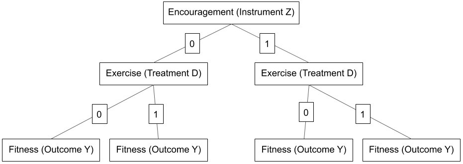
Compliers and non-compliers
- Compliers: Exercise (take treatment, D = 1) if encouraged (Z = 1), do not exercise (take control, D = 0) if not encouraged (Z = 0)
- In short: they do as they are told to!
- Non-compliers (e.g. Angrist et al. 1996)
- Never takers: Do not exercise (D = 0) regardless of encouragement (Z = 1 or Z = 0)
- Do not take treatment regardless of assignment status
- Always takers: Exercise (D = 1) regardless of encouragement (Z = 1 or Z = 0)
- Take the treatment regardless of assignment status
- Defiers: Do the opposite of encouragement
- Take the treatment when assigned to control and vice versa
- D = 1 when Z = 0; D = 0 when Z = 1
- Never takers: Do not exercise (D = 0) regardless of encouragement (Z = 1 or Z = 0)
Instrumental variables: Exercise
- Q: Below we have our decision tree again. In which leaf(s) (1-4 from left to right) would we find people that belong to the different categories namely compliers and non-compliers whereby the latter are divided into never takers, always takers and defiers (e.g. Dunning 2009, 2702f)?
- Beware: Non-compliance may occur in most seemingly perfect randomized experiments!
- Q: Use the aspirin example and explain the four types of experimental participants.
- Q: Knowing the above, why are “manipulation checks” in experiments so important?
CACE/LATE and ITT
- IV analysis allows us to estimate the complier average causal effect (CACE)
- Average effect among those induced to take (and not to take) treatment by randomized encouragement
- is also a local average treatment effect (LATE)
- Estimand local because only defined for sub population: the compliers
- We can also estimate the Intention-to-treat effect (ITT)
- Another interesting quantity
- Effect of encouragement Z on fitness Y (Randomly assigned and therefore identified)
Identification assumption(s): Update Lousdal 2018
- Lousdal (2018, 2-4) provides one of the best summaries of IV assumptions (+ lucid explanations)
- Three basic assumptions (A1-3) and a fourth one (A4) [ \(X\) replaced with \(D\) on slides ]
- A variable \(Z\) is an instrument if it meets the following three assumptions:
- The relevance assumption (A1): The instrument \(Z\) has a causal effect on \(D\).
- The exclusion restriction assumption (A2): \(Z\) affects the outcome \(Y\) only through \(D\).
- The exchangeability assumption (A3): \(Z\) does not share common causes with the outcome \(Y\)
- Also called independence assumption, ignorable treatment assignment, no confounding for effect of \(Z\) on \(Y\)
- The monotonicity or no defiers assumption (A4): There are no defiers (cf. Lousdal 2018, 3-4; Dunning 2009, 2704)
- If no defiers exist (A4), then the only subpopulation in which \(Z\) can affect \(D\) is the compliers, i.e., effect of \(Z\) on \(Y\) will only stem from the group of compliers
- A1-4 allow us to estimate local average treatment effect (LATE) also called complier average causal effect (CACE)
- Problem that remains (for decision makers): We can not identify the compliers individually (differentiate from always/never takers)
Estimation: Two stages
- First stage: \(\hat{D}_{i} = \alpha + \delta Z_{i} + \mathbf{X}_{i}\mathbf{\beta}\)
- Regress treatment \(D\) on instrument \(Z\)
- Second stage: \(y_{i} = \gamma + \theta \hat{D}_{i} + \mathbf{X}_{i}\mathbf{\beta} + \epsilon_{i}\)
- Regress outcome \(Y\) on the predicted values of the first regression
- Conceptually:
- predicted values reflect the variation in treatment \(D\) that is explained by the instrument \(Z\)
- this left-over variation is exogenous so we can estimate it’s causal effect on \(Y\)
- Stages often implemented in single function, e.g.
ivreg()in R
Limitations (and Strengths) (1)
Requires strong assumptions (can be partially validated with data)
As-if random (independence) IV assumption
- Show \(Z\) to be uncorrelated with pretreatment covariates
- Use a priori reasoning and detailed knowledge of empirical context
- Observational studies: Often matter of opinion (“less plausible” to “more plausible”)
Additional issues with use of multiple regression models
- Concern about endogeneity of single treatment variable (counfounding)
- Researchers add covariates to condition but forget to discuss their potential endogeneity
- Recommendation: also report regression without covariates (the latter can be harmful)
- Truly random instruments may not show strong correlation with (endogenous) treatment
- Small-sample bias can arise and its recommended to report “reduced-form” results (i.e., ITT effect namely \(D\) on \(Z\))
- Generally, be careful in extrapolating results and validate the linear regression model itself
- Concern about endogeneity of single treatment variable (counfounding)
Limitations (and Strengths) (2)
- Important!
- Neither core criteria for a valid instrumental variable, i.e., …
- … \(Z\) is statistically independent of unobserved causes of the dependent variable and…
- …affects the dependent variable only through its effect on the endogenous treatment \(D\),…
- …are directly testable from data
- Neither core criteria for a valid instrumental variable, i.e., …
- We have to defend these assumptions using evidence and reasoning but be careful especially outside of experimental studies!
Examples & Further reading
- Does lower turnout reduce the vote share of the democratic party? (Hansford and Gomez 2010)
- Outcome Y: Democratic vote share
- Treatment D: Turnout
- Instrument Z: Rainfall decreases turnout on election day
- LATE: Effect of turnout on vote share among the counties discouraged to vote by rain on election day
- The Slave Trade and the Origins of Mistrust in Africa (Nunn and Wantchekon 2011)
- Outcome Y: Trust
- Treatment D: Slave trade (numbers between 1400 and 1900)
- Instrument Z: Distance to the coast
- Lifetime Earnings and the Vietnam Era Draft Lottery: Evidence from Social Security Administrative Records (Angrist 1990)
- Outcome Y: Civilian earnings
- Treatment D: Veteran status
- Instrument Z: Draft lottery
Exercise: Screening & Breast cancer (Dunning 2009)
- Homework: Read through Dunning’s example and explain the logic of IV analysis using Table 1 below.
- Invitation (Z), screening (D), cancer (Y): Exemplary calculation assuming presence and absence of certain groups (e.g., compliers etc.)
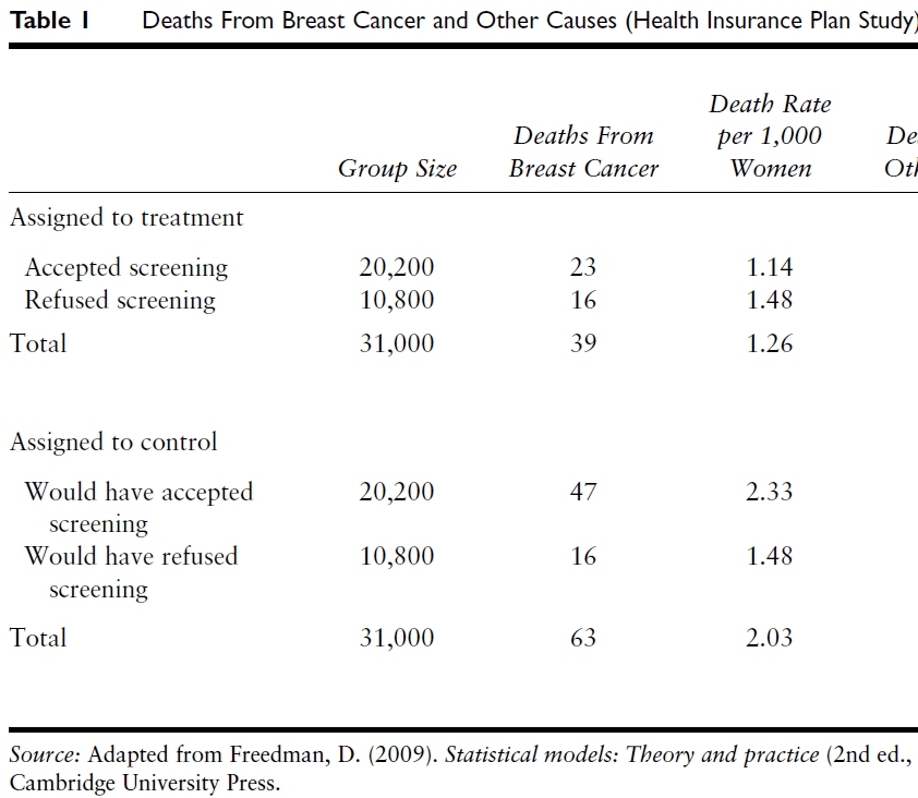
Summary
IVs help confront the problem of confounding
IV logic is helpful even if you don’t find a good instrument
- It makes us think about compliers, always takers etc., i.e., why people might take the treatment or not
Experimental studies: Assignment can be seen as an IV of actually taking treatment/control
Observational studies: Often very hard to find good, credible instrumental variables
- Assumptions have to be convincing and there aren’t many convincing applications
Intro
15 Minutes for the evaluation!
Questions and answer document: See this file!
Retake: IV
- Why might we want to use IV? (e.g., vs. matching + conditional independence assumption)
- Why not use a logistic regression to predict \(D\) with \(Z\)?
- What are the IV assumptions that identify the LATE/CACE?
- IV homework!
Regression discontinuity design (based on Cattaneo et al. 2019)
IV questions
- Why might we want to use IV? (e.g., vs. matching + conditional independence assumption)
- Kern & Hainmueller 2009 Example
- West German television exposure \(D\) \(\rightarrow\) support for East German regime \(Y\)
- Instrument: Living in Dresden \(Z\)
- Reverse causation \(D \leftarrow Y\)
- e.g., people do or do not seek access to West German television because of their low or high support of the East German regime
- Confounding \(D \leftarrow X \rightarrow Y\)
- e.g., having relatives in West Germany \(X\) might affect both one’s West German television exposure \(D\) and support for East German regime \(Y\) (we can think of different mechanisms)
- Kern & Hainmueller 2009 Example
Identification assumption(s): Update Lousdal 2018
- Lousdal (2018, 2-4) provides one of the best summaries of IV assumptions (+ lucid explanations)
- Three basic assumptions (A1-3) and a fourth one (A4) [ \(X\) replaced with \(D\) on slides ]
- A variable \(Z\) is an instruments if it meets the following three assumptions:
- The relevance assumption (A1): The instrument \(Z\) has a causal effect on \(D\).
- The exclusion restriction assumption (A2): \(Z\) affects the outcome \(Y\) only through \(D\).
- The exchangeability assumption (A3): \(Z\) does not share common causes with the outcome \(Y\)
- Also called independence assumption, ignorable treatment assignment, no confounding for effect of \(Z\) on \(Y\)
- The monotonicity or no defiers assumption (A4): There are no defiers (cf. Lousdal 2018, 3-4; Dunning 2009, 2704)
- If no defiers exist (A4), then the only subpopulation in which \(Z\) can affect \(D\) is the compliers, i.e., effect of \(Z\) on \(Y\) will only stem from the group of compliers
- A1-4 allow us to estimate local average treatment effect (LATE) also called complier average causal effect (CACE)
- Problem that remains (for decision makers): We can not identify the compliers individually (differentiate from always/never takers)
Identification assumption(s): Examples
- The relevance assumption (A1): The instrument \(Z\) has a causal effect on \(D\)
- “Given that most people in the Dresden district were cut off from West German television broadcasts, not living in the Dresden district is highly correlated with exposure to West German television.” (Kern & Hainmueller 2009, 385)
- The exclusion restriction assumption (A2): \(Z\) affects the outcome \(Y\) only through \(D\).
- Threat: Alternative mechanisms/paths, e.g., Living in Dresden \(Z\) \(\rightarrow\) Living conditions \(X\) \(\rightarrow\) Political support \(Y\)
- See Kern & Hainmueller (2009, Section 3.2.2) for arguments why assumption holds condition on covariates. (highlight similarity of Dresden and control districts in Fig.2)
- The exchangeability assumption (A3): \(Z\) does not share common causes with the outcome \(Y\)
- Threat: “East Germans who desired to watch West German television might have moved away from the Dresden district. If interest in West German television was correlated with regime support, which seems likely, this kind of sorting behavior would invalidate our instrument” (Kern & Hainmueller 2009, 386)
- See Kern & Hainmueller (2009, Section 3.2.3) for arguments why assumption holds condition on covariates (highlight low mobility).
- The monotonicity or no defiers assumption (A4): There are no defiers (cf. Lousdal 2018, 3-4; Dunning 2009, 2704)
- “It is highly unlikely that there were East Germans who would have watched West German television if they had lived in Dresden but who would not have watched West German television if they had not lived in Dresden.” (Kern & Hainmueller 2009, 384)
Homework (1): Screening & Breast cancer
1960s: Health Insurance Plan (HIP) clinical trial studied effects of screening \(D\) for breast cancer \(Y\) (Dunning 2009)
- Assigned-to-treatment group (or treatment group): ~31,000 women between 40 and 64 years invited for annual clinical visits and mammographies (X-rays designed to detect breast cancer)
- Control group: ~31,000 women received status quo health care
Instrument: Invitation for screening \(Z\) issued at random
- Women in assigned-to-treatment group were just like the women who were not, up to random error
Table 1 (next slide) shows death rates from breast cancer 5 years after trial
Homework: Read through Dunning’s (2009) example and explain the different comparisons we can make and the logic of IV analysis using Table 1 below.
- Exemplary calculation assuming presence of Compliers and Never Takers (but absence of Always Takers/Defiers)
Homework (2): Screening & Breast cancer
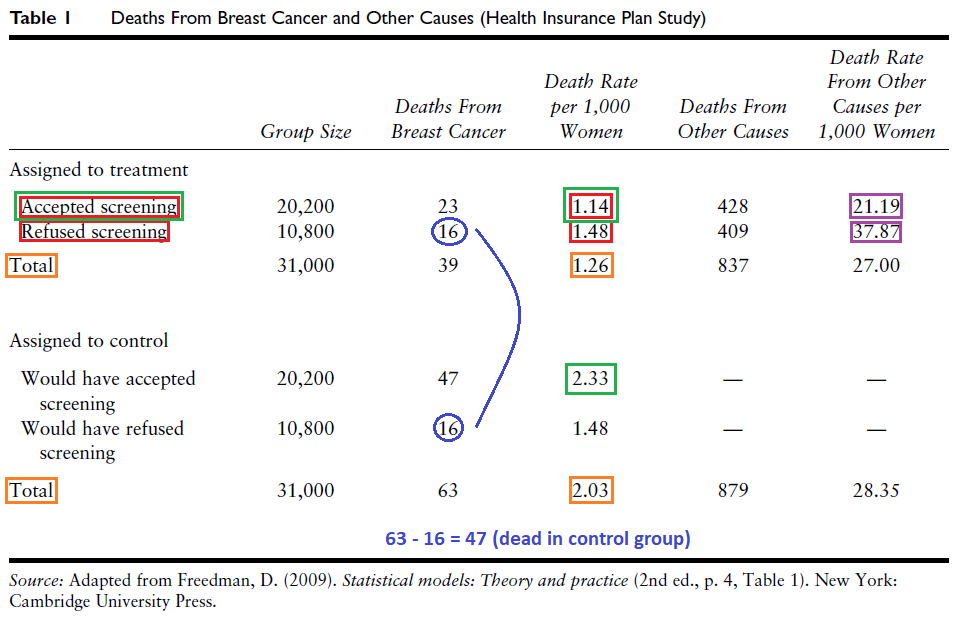
Homework (3): Screening & Breast cancer
- Naive comparison (red): Compare women who received screening with those that refused (Est.: -0.34)
- Problem: Self-selection into treatment, i.e., women who screened systematically different (richer, better-educated)
- Problem: richer, better-educated more prone to breast cancer [Explanation: fewer children]
- Correct, experimental comparison (orange): Compare women randomly invited (whether or not they were actually screened) to the whole control group
- Intention-to-treat analysis: Shows strong effect in relative terms (effect: -0.77)
- 1.26 (assignment-to-treatment group) - 2.03 (control group)
- Probably understates effect because one third (10800) in treatment group not screened
- Intention-to-treat analysis: Shows strong effect in relative terms (effect: -0.77)
- What was the effect of screening on women in the treatment group who accepted screening (green)?
- Control group (total): Can not differentiate compliers/never takers (neither receives treatment when assiged to control) [we assume only the two groups - compliers & never takers are present]
- Treatment group: ~2/3 (20200) accepted screening \(\rightarrow\) because of random assignment mix of never takers and compliers should be same in control group (~2/3 would have accepted screening in both)
- IV analysis compares death rates of compliers in treatment [1, green, observable!] and control [2]
- Calculate [2]: Rate of NTs same in both groups (blue circle, 16) -> 63 - 16 = 47 dead compliers in control group
- Calculate death rates of compliers in treatment and control:
(23/20200)*1000 = 1.14;(47/20200)*1000 = 2.33 - LATE/CATE: 1.14 - 2.33 = -1.19
- Calculate death rates of compliers in treatment and control:
- Assumption(s): No Always Takers, i.e., no women screened in the control group (we could adjust for double cross-over!) and absence of defiers
IV questions
- Why might we want to use IV? (e.g., vs. matching + conditional independence assumption)
- Kern & Hainmueller 2009 Example
- West German television exposure \(D\) \(\rightarrow\) support for East German regime \(Y\)
- Instrument: Living in Dresden \(Z\)
- Reverse causation \(D \leftarrow Y\)
- e.g., people do or do not seek access to West German television because of their low or high support of the East German regime
- Confounding \(D \leftarrow X \rightarrow Y\)
- e.g., having relatives in West Germany \(X\) might affect both one’s West German television exposure \(D\) and support for East German regime \(Y\) (we can think of different mechanisms)
- Kern & Hainmueller 2009 Example
Identification assumption(s): Update Lousdal 2018
- Lousdal (2018, 2-4) provides one of the best summaries of IV assumptions (+ lucid explanations)
- Three basic assumptions (A1-3) and a fourth one (A4) [ \(X\) replaced with \(D\) on slides ]
- A variable \(Z\) is an instruments if it meets the following three assumptions:
- The relevance assumption (A1): The instrument \(Z\) has a causal effect on \(D\).
- The exclusion restriction assumption (A2): \(Z\) affects the outcome \(Y\) only through \(D\).
- The exchangeability assumption (A3): \(Z\) does not share common causes with the outcome \(Y\)
- Also called independence assumption, ignorable treatment assignment, no confounding for effect of \(Z\) on \(Y\)
- The monotonicity or no defiers assumption (A4): There are no defiers (cf. Lousdal 2018, 3-4; Dunning 2009, 2704)
- If no defiers exist (A4), then the only subpopulation in which \(Z\) can affect \(D\) is the compliers, i.e., effect of \(Z\) on \(Y\) will only stem from the group of compliers
- A1-4 allow us to estimate local average treatment effect (LATE) also called complier average causal effect (CACE)
- Problem that remains (for decision makers): We can not identify the compliers individually (differentiate from always/never takers)
Identification assumption(s): Examples
- The relevance assumption (A1): The instrument \(Z\) has a causal effect on \(D\)
- “Given that most people in the Dresden district were cut off from West German television broadcasts, not living in the Dresden district is highly correlated with exposure to West German television.” (Kern & Hainmueller 2009, 385)
- The exclusion restriction assumption (A2): \(Z\) affects the outcome \(Y\) only through \(D\).
- Threat: Alternative mechanisms/paths, e.g., Living in Dresden \(Z\) \(\rightarrow\) Living conditions \(X\) \(\rightarrow\) Political support \(Y\)
- See Kern & Hainmueller (2009, Section 3.2.2) for arguments why assumption holds condition on covariates. (highlight similarity of Dresden and control districts in Fig.2)
- The exchangeability assumption (A3): \(Z\) does not share common causes with the outcome \(Y\)
- Threat: “East Germans who desired to watch West German television might have moved away from the Dresden district. If interest in West German television was correlated with regime support, which seems likely, this kind of sorting behavior would invalidate our instrument” (Kern & Hainmueller 2009, 386)
- See Kern & Hainmueller (2009, Section 3.2.3) for arguments why assumption holds condition on covariates (highlight low mobility).
- The monotonicity or no defiers assumption (A4): There are no defiers (cf. Lousdal 2018, 3-4; Dunning 2009, 2704)
- “It is highly unlikely that there were East Germans who would have watched West German television if they had lived in Dresden but who would not have watched West German television if they had not lived in Dresden.” (Kern & Hainmueller 2009, 384)
Homework (1): Screening & Breast cancer
1960s: Health Insurance Plan (HIP) clinical trial studied effects of screening \(D\) for breast cancer \(Y\) (Dunning 2009)
- Assigned-to-treatment group (or treatment group): ~31,000 women between 40 and 64 years invited for annual clinical visits and mammographies (X-rays designed to detect breast cancer)
- Control group: ~31,000 women received status quo health care
Instrument: Invitation for screening \(Z\) issued at random
- Women in assigned-to-treatment group were just like the women who were not, up to random error
Table 1 (next slide) shows death rates from breast cancer 5 years after trial
Homework: Read through Dunning’s (2009) example and explain the different comparisons we can make and the logic of IV analysis using Table 1 below.
- Exemplary calculation assuming presence of Compliers and Never Takers (but absence of Always Takers/Defiers)
Homework (2): Screening & Breast cancer
Homework (3): Screening & Breast cancer
- Naive comparison (red): Compare women who received screening with those that refused (Est.: -0.34)
- Problem: Self-selection into treatment, i.e., women who screened systematically different (richer, better-educated)
- Problem: richer, better-educated more prone to breast cancer [Explanation: fewer children]
- Correct, experimental comparison (orange): Compare women randomly invited (whether or not they were actually screened) to the whole control group
- Intention-to-treat analysis: Shows strong effect in relative terms (effect: -0.77)
- 1.26 (assignment-to-treatment group) - 2.03 (control group)
- Probably understates effect because one third (10800) in treatment group not screened
- Intention-to-treat analysis: Shows strong effect in relative terms (effect: -0.77)
- What was the effect of screening on women in the treatment group who accepted screening (green)?
- Control group (total): Can not differentiate compliers/never takers (neither receives treatment when assiged to control) [we assume only the two groups - compliers & never takers are present]
- Treatment group: ~2/3 (20200) accepted screening \(\rightarrow\) because of random assignment mix of never takers and compliers should be same in control group (~2/3 would have accepted screening in both)
- IV analysis compares death rates of compliers in treatment [1, green, observable!] and control [2]
- Calculate [2]: Rate of NTs same in both groups (blue circle, 16) -> 63 - 16 = 47 dead compliers in control group
- Calculate death rates of compliers in treatment and control:
(23/20200)*1000 = 1.14;(47/20200)*1000 = 2.33 - LATE/CATE: 1.14 - 2.33 = -1.19
- Calculate death rates of compliers in treatment and control:
- Assumption(s): No Always Takers, i.e., no women screened in the control group (we could adjust for double cross-over!) and absence of defiers
Appendix D: Effect size/uncertainty, mediation and heterogeneity
Effect size: Starter
Studies in sociology and political science often make a statement about statistical significance but rarely about actual effect size (but it’s getting better!).
Q: What is the difference between statistical significance and effect size? What is the source of uncertainty in our effect estimates?
‘Sing me a song with social significance’: The (mis) use of statistical significance testing in European sociological research (2017)
- “we analyse the ritual of null hypothesis significance testing among the European sociologists. The focus is on the distinction between statistical significance and substantive, sociological significance. We review all articles published in the European Sociological Review between 2000–2004 and 2010–2014 that use regression models (N = 356). Our main aim is to determine whether the authors discuss the effect size of their findings and distinguish substantive from statistical significance. We apply a five-item questionnaire to each article and find that about half of the articles erroneously interpret a statistically insignificant coefficient as a zero effect, while only one in three engage in a discussion of the substantive meaning of the effect sizes. Moreover, our findings show a negative trend in the practice of significance testing over the past 15 years. These results are similar to those of the comparable review in the field of economics.” (Bernardi et al. 2017)
Effect size (1)
- Effect size: In causal research effect often = difference in means of \(Y\) between treatment and control group
- Q: Is it easier to judge difference (effect size) on income scale (in euros) or on a trust scale (4 levels)?
–
Yes, income!
Examples (in my own research):
- Victimization (0,1) on generalized trust (0-10): ~0.6 (naive estimate)
- Fake vs. real source (Nachricten 360/Tagesschau) on belief (0-6): 0.62 (comparable to similar studies)
“Vague” scales
- Approach 1: What effect sizes did previous studies with the same outcome scale identify?
- Approach 2: What are the biggest differences we can observe on that outcome scale?
- …between units (e.g., males and females)
- …within units (e.g., individual’s drop in life satisfaction scale after child’s death)
Effect size (2)
- Approach 3: Standardization
data$trust.2006 <- (data$trust.2006 - mean(data$trust.2006))/sd(data$trust.2006)- Q: What does the above code do?
- Standardize outcome variable to mean = 0 and standard deviation = 1
- New unit on standardized variable = standard deviations
- Try this app to understand the impact standardizing has on a variable
- Possible assumption: Standardized variable = normally distributed (see Figure on the right)
- Then we know more or less how many people are located within 1 SD
- e.g. a difference of 1 standard deviation on the outcome scale between treated/control could be regarded as strong (“a lot of people shifting positions”)
- Try using a combination of Approach 1, 2 and 3 in your own research
Effect uncertainty (1)
- Objective: estimate causal effect \(\theta\), e.g., effect of education on income in a (target) population \(P\)
- \(P\) could be Mannheim students, German citizens, immigrants etc.
- Steps: Define population \(P\) → collect sample \(S\) from population → produce estimate \(\hat{\theta}\)
- Estimate comes with uncertainty, i.e., we don’t know how far \(\hat{\theta}\) is from true population parameter \(\theta\)
- Dominant perspective: Uncertainty about population parameters is induced by random sampling from the population
- Typically assume that sample comprises only a small fraction of the population of interest
- Sampling perspective…
- …makes sense when data can be regarded as small random subset of population of interest (e.g., ALLBUS data)
- …makes less sense when we have data on the whole population (e.g., comparing countries): then we know our estimates with certainty!
Effect uncertainty (2)
Frequentist paradigm: In theory, we draw repeated samples \((S_{1}, S_{2}, S_{3}, ...)\) from population \(P\)
In each sample we calculate the quantity of interest resulting in a vector of estimates: \((\hat{\theta}_{S1}, \hat{\theta}_{S2}, \hat{\theta}_{S3}, ...)\)
- The distribution of these estimates is called sampling distribution…
- …and is the distribution of the \(\hat{\theta}'s\) that we get across these different samples
Central limit theorem (CLT): Roughly states that sampling distribution (given certain conditions) approaches a normal distribution
In reality, we normally only observe one sample but we can still assume (CLT!) that the sampling distribution would look like a normal distribution (or a t-distribution)
Classic standard errors (SEs) [and also confidence intervals]: are based on this frequentist logic and are designed to capture sampling variation
- e.g., “sample mean’s standard error is the standard deviation of the set of means that would be found by drawing an infinite number of repeated samples from the population and computing a mean for each sample” (Wikipedia)
Effect uncertainty (3): Standard errors
Standard error (SE): the standard deviation (SD) of the sampling distribution of a statistic, e.g., of our causal effect of interest
- Standard deviation (SD) is a measure of the amount of variation or dispersion of a set of values
Sample mean as ‘simple’ example: Mean \(\bar{x}\) is quantity of interest and the samples are uncorrelated
- Standard error of the sample mean (also called SEM): SE = \(\sigma_{\bar{x}}={\frac{\sigma }{{\sqrt{n}}}}\)
- \(\sigma\) \((=\sqrt{\sigma^{2}})\)): standard deviation of the population distribution of \(x\)
- \(n\): number of units in the sample (sample size)
- \(\sigma\) seldomly known so we replace it with the sample standard deviation \(s = \sqrt{\frac{1}{n} \sum_{i=1}^{n} (x_{i} - \bar{x})^2}\)
- Implication of formula \((\sqrt{n})\): Sample size must be multiplied by 4 to achieve half the SE (cost-benefit tradeoffs)
- Standard error of the sample mean (also called SEM): SE = \(\sigma_{\bar{x}}={\frac{\sigma }{{\sqrt{n}}}}\)
If sampling distribution is normally distributed, sample mean, standard error, and quantiles of the normal distribution can be used to calculate confidence intervals for the true population mean
Same logic applies to other quantities of interest, e.g., difference in means (causal effect etc.), estimates from linear regression model etc.
Uncertainty: Sampling-based vs. design-based (1)
Sampling-based uncertainty: stems from the fact that we only observe a subset of the population (Abadie et al. 2020)
Table I: finite population consisting of \(n\) units with each unit characterized by a pair of variables \(Y_{i}\) and \(Z_{i}\), with inclusion of unit \(i\) in a sample encoded by the binary variable \(R_{i} \in \{0,1\}\)
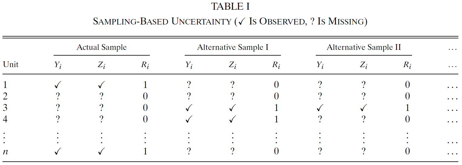
- Sampling-based inference uses information about the process that determines the sampling indicators \(R_{1}, ..., R_{n}\) to assess the variability of estimators across different samples (Table I shows three samples)
Uncertainty: Sampling-based vs. design-based (2)
Design-based uncertainty: “arises when the parameter of interest is defined in terms of the unobserved outcomes that some units would attain under a certain intervention” (Abadie et al. 2020, 266)
Table II: scenario in which we observe, for each unit in the population, the value of one of two potential outcome variables, either \(Y^{∗}_{i}(1)\) or \(Y^{∗}_{i}(0)\); \(X_{i}\in\{0,1\}\) indicates which potential outcome we observe

- Design-based inference uses information about the process that determines the assignments \(X_{1}, ..., X_{n}\) to assess the variability of estimators across different samples (Table II shows three samples)
Uncertainty: Sampling-based vs. design-based (3)
We face a missing data process that may combine features of these two examples
- Some units not included in the sample at all (1) and with some of the variables (e.g., treatment) not observed for the sampled units (2)
Articulating both exact nature of the estimand of interest and the source of uncertainty that makes an estimator stochastic is a crucial first step to valid inference (Abadie et al. 2020, 266)
Useful to distinguish…
- …cases where uncertainty stems solely from not observing all units in the population of interest
- …cases where the uncertainty stems (partially) from unobservability of some of the potential outcomes
When interest is descriptive (e.g., mean age in population, income difference between men and women) we are only concerned with sampling-based uncertainty
- Causal estimands (e.g., causal effect of gender on income) require consideration of both uncertainties
Internal vs. external validity
We can now also return to the concepts of internal vs. external validity
Abadie et al. (2020, 271)’s distinction between sampling-based and design-based uncertainty suggests a definition of these concepts
“Internal validity bears on the question of whether \(E[\theta|\mathbf{R},N_{1},N_{0}]\) is equal to \(\theta^{causal,sample}\). This relies on random assignment of the treatment. Whether or not the sampling is random is irrelevant for this question because \(\theta^{causal,sample}\) conditions on which units were sampled.” (Abadie et al. 2020, 271)
- \(\mathbf{R}\): Population \(n\)-vector with \(i\)th element equal to \(R_{i}\) (units with \(R_{i}=1\) are included in the sample)
- \(N_{1},N_{0}\): Number of units in treatment and control
“External validity bears on the question of whether \(E[\theta^{causal,sample}|N_{1},N_{0}]\) equal to \(\theta^{causal}\) [population!]. This relies on the random sampling assumption and does not require that the assignment is random” (Abadie et al. 2020, 271)
“However, for \(\hat{\theta}\) to be a good estimator of \(\theta^{causal}\), which is often the most interesting estimand, we need both internal and external validity, and thus both random assignment and random sampling.” (Abadie et al. 2020, 271)
Effect Mediation & causal mechanisms (1)
Whether variable \(A\) has a causal effect on variable \(B\) vs. explain how causal relationship between \(A\) and \(B\) arises
Causal mechanism (CM): “a process in which a causal variable of interest, i.e., a treatment variable, influences an outcome” (Imai et al. 2011, 765)
- Identification of CM requires specification of an intermediate variable or a mediator \(M\) that lies on the causal pathway between treatment \(T\) (= \(D\)) and outcome variable \(Y\)
Q: Can you think of any examples of mediators \(M\) that mediate a causal relationship between \(D\) and \(Y\)?
Contributions (Imai et al. 2011, 766): “commonly used statistical methods [cf. Baron & Kenny 1986] rely upon untestable assumptions and are often inappropriate even under those assumptions” (Imai et al. 2011, 764)
- Present minimum set of assumptions required to quantify causal mediation effect under standard designs (experimental, observational) (and provide methods in R)
- Develop method of assessing the sensitivity of conclusions to potential violations of (untestable) key assumptions (-Sensitivity analysis formally quantifies degree to which empirical findings rely upon the key assumptions-)
- Offer alternative research designs that enable identification of causal mechanisms under less stringent assumptions
Effect Mediation & causal mechanisms (2)
- Causal mechanism: “process whereby one variable \(T\) [= \(D\)] causally affects another \(Y\) through an intermediate variable or a mediator \(M\) that operationalizes the hypothesized mechanism” (Imai et al. 2011, 768)
- e.g., Causal effect of \(\text{media framing }(T)\) (neg. immigration vs. neutral story) on \(\text{attitudes toward immigration }(Y)\) is transmitted by respondents’ \(\text{anxiety }(M)\) (High vs. low) (Brader et al. 2008)
- Media effects may operate through changes in anxiety OR NOT
- Inferential goal: Decompose the causal effect of \(\text{media framing }(T)\) into the indirect effect, which represents the hypothesized causal mechanism, and the direct effect, which represents all the other mechanisms
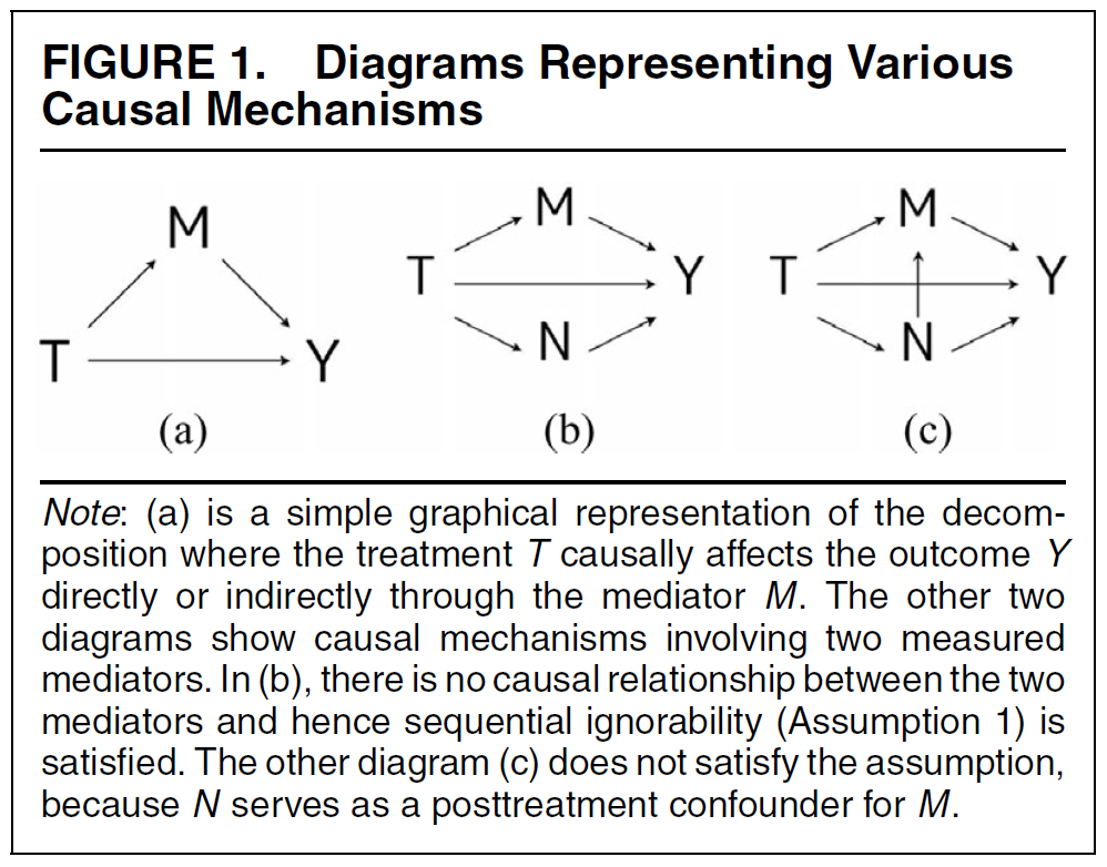
- Q: Where do we see indirect and direct effect in Fig. 1a on the right? What do Fig. 1b/c show?
Effect Mediation & causal mechanisms (3)
Example of Brader et al. (2008)
- \(T\): media framing; \(t = \text{{0/neutral immigration story, 1/neg. immigration story}}\)
- \(M\): level of anxiety; \(m = \text{{0/low, 1/high}}\)
- \(Y\): immigration attitude
\(M_{i}(t)\): potential value of mediator for unit \(i\) under the treatment status \(T_{i}=t\) (Q: \(M_{i}(1)=?\) )
\(Y_{i}(t,m)\): potential outcome that would result if the treatment and mediating variables equal \(t\) and \(m\)
- e.g., \(Y_{i}(1,1)\): potential outcome/opinion of individual \(i\) given she has high anxiety and previously got the neg. immigration story (Q: \(Y_{i}(0,1)=?\) )
Difference to usual situation
- The observed outcome \(Y_{i}\) now depends on two things.. the treatment status and level of mediator observed under treatment status, i.e., \(Y_{i}(T_{i},M_{i}(T_{i}))\)
Effect Mediation & causal mechanisms (4)
- Total unit treatment effects
- \(\tau_{i}=Y_{i}(1,M_{i}(1))−Y_{i}(0,M_{i}(0))\):
- e.g., effect of media framing \(T\) on immigration attitudes \(Y\) (“ignoring” \(M_{i}\))
- BUT we want to divide this into direct and indirect effect
- \(\tau_{i}=Y_{i}(1,M_{i}(1))−Y_{i}(0,M_{i}(0))\):
- Direct effects of the treatment for each unit \(i\) and each treatment status \(t=0,1\)
- \(\zeta_{i}(t)\equiv Y_{i}(1,M_{i}(t))−Y_{i}(0,M_{i}(t))\)
- Example: \(\zeta_{i}(1)\) represents the difference between immigration opinions under treatment \((t = 1 = \text{0/neg. immigration story})\) and control \((t = \text{0/neutral immigration story})\) holding \(M (\text{anxiety level})\) constant at the level that would be realized under treatment \((t = 1)\)
- The direct effect \(\zeta_{i}(t)\) equals the causal effect of the treatment \(T\) on the outcome \(Y\) that is not transmitted by the hypothesized mediator \(M\)
- The direct effect \(\zeta_{i}(t)\) equals the causal effect of the treatment \(T\) on the outcome \(Y\) that is not transmitted by the hypothesized mediator \(M\)
- Q: What is \(\zeta_{i}(0)\)?
Effect Mediation & causal mechanisms (5)
- Indirect causal mediation effects for each unit \(i\) and each treatment status \(t=0,1\)
- \(\delta_{i}(t)\equiv Y_{i}(t,M_{i}(1))−Y_{i}(t,M_{i}(0))\):
- Example: \(\delta_{i}(1) = Y_{i}(1,M_{i}(1)) - Y_{i}(1,M_{i}(0))\) represents the difference between the two potential immigration opinions for subject \(i\) under \(t = 1 = \text{0/neg. immigration story}\) but changing the mediator \(M\)
- \(Y_{i}(1,M_{i}(1))\): is the (observable) immigration opinion if she views the neg. immigration news story
- \(Y_{i}(1,M_{i}(0))\): is her immigration opinion under the counterfactual scenario where subject \(i\) still viewed the neg. immigration story but her anxiety level is as if the subject viewed the control (neutral) news story
- Difference between these two potential outcomes \((Y_{i}(1,M_{i}(1)) \text{ and } Y_{i}(1,M_{i}(0)))\) represents the effect of the change in the mediator that would be induced by the treatment, while the direct impact of the treatment is suppressed holding its value constant (here at \(t = 1\))
- Q: \(\delta_{i}(0)=?\)
Effect Mediation: Estimation
- Aim: Estimate…
- …average (indirect) causal mediation effects (ACME) \(\bar\delta(t)\)
- …average direct effects (ADE) \(\bar\zeta(t)\)
- ATE \(\bar\tau\) equals the sum of ACME and ADE
- Goal is to decompose the ATE into the ACME and ADE and then assess the relative importance of the hypothesized mechanism
- Key insight
- Both the direct and indirect effects contain a potential outcome that would never be realized under these designs
- Therefore neither quantity can be identified even in randomized experiments (where we randomize both \(T\) and \(M\)), let alone observational studies
- Under these designs the ATE is identified, but the ACME and ADE are not
- We need additional assumptions!
Effect Mediation: Identification assumptions (1)
- Assumption 1: sequential ignorability (required under standard designs \(\ast)\)
- \(\ast:\) Treatment assignment is either randomized or assumed to be random given the pretreatment covariates
- See Imai et al. (2011, 770) for formula of sequential ignorability assumption
- \(X_{i}\): Observed pretreatment confounders for unit \(i\) (e.g., respondent’s gender and race in the media framing study)
- sequential ignorability makes two ignorability assumptions sequentially
- Given the observed pretreatment confounders, the treatment assignment is assumed to be statistically independent (ignorable) of potential outcomes and potential mediators
- Assumption normally holds in experiments as in the Brader et al. (2008) example discussed here
- Also called no-omitted-variable bias, unconfoundedness, etc.
- Observed mediator is ignorable given the actual treatment status and pretreatment confounders
- Example on next slide!
Effect Mediation: Identification assumptions (2)
Example for sequential ignorability (1) and (2)
- because news stories are randomly assigned to subjects, the first part of Assumption 1 will hold even without conditioning on any pretreatment covariates \(X_{i}\)
- implies that there are no unmeasured pretreatment or posttreatment covariates that confound the relationship between the levels of anxiety \(M\) and immigration opinions \(Y\)
- That is a strong assumption even in randomized experiments..
- Would require measurement of complete set of covariates that affect both anxiety and immigration opinions, and they all must not be affected by the treatment
- Violation, e.g., if both anxiety and immigration opinions are affected by fear disposition or ideology
If sequential ignorability holds we can identify ACME and ADE [+ Assumption 2: consistency assumption, see discussion in Imai et al. (2011, 782)]
Imai et al. (2011) also provide R code to conduct causal mediation analysis
- See package on github: https://github.com/kosukeimai/mediation
Appendix: Only relevant when discussed during the lecture
Standard Errors (1): Clustering
- Calculation of standard errors can be complicated when units are clustered, e.g., students in school classes (Cameron and Miller 2015, Abadie et al. 2017)
- Clustering is a design problem (Abadie et al. 2017)
- Sampling design issue: When sampling follows two stage process, 1st stage: Clusters sampled randomly from population of clusters; 2nd stage: Units sampled randomly from the sampled clusters
- e.g., students sampled from sample of school classes
- Clustering adjustment is justified because there are clusters in the population that we do not see in the sample
- Experimental design issue: When clusters of units, rather than units, are assigned to a treatment
- e.g., unit = students but randomization happens on the level of school classes
- Sampling design issue: When sampling follows two stage process, 1st stage: Clusters sampled randomly from population of clusters; 2nd stage: Units sampled randomly from the sampled clusters
- Clustering will in general be justified, if the sampling or assignment varies systematically with groups in the sample (Abadie et al. 2017, 2) → Look out for future developments
Standard Errors (2): Clustering
- Further reading
- Cameron, A. Colin, and Douglas L. Miller. 2015. “A Practitioner’s Guide to Cluster-Robust Inference.” The Journal of Human Resources 50 (2): 317–72.
- Abadie, Alberto, Susan Athey, Guido Imbens, and Jeffrey Wooldridge. 2017. “When Should You Adjust Standard Errors for Clustering?” arXiv [math.ST]. arXiv. http://arxiv.org/abs/1710.02926.
- Bertrand, Marianne, Esther Duflo, and Sendhil Mullainathan. 2004. “How Much Should We Trust Differences-In-Differences Estimates?” The Quarterly Journal of Economics 119 (1): 249–75.
- King, Gary, and Margaret E. Roberts. 2015. “How Robust Standard Errors Expose Methodological Problems They Do Not Fix, and What to Do About It.” Political Analysis: An Annual Publication of the Methodology Section of the American Political Science Association 23 (2): 159–79.
- Also see this nice tutorial by Clay Ford
- Abadie et al. 2020: “alternative framework for the interpretation of uncertainty in regression analysis regardless of whether a substantial fraction of the population or even the entire population is included in the sample”
- Sampling-based vs. design-based uncertainty
Intro
Slides: https://paulcbauer.github.io/research_design_2022/lecture_14.html
Causal mediation analysis (rest)
Review of material
Exam
Questions!
Causal Mediation Analysis
Effect Mediation: Estimation
- Aim: Estimate…
- …average (indirect) causal mediation effects (ACME) \(\bar\delta(t)\)
- …average direct effects (ADE) \(\bar\zeta(t)\)
- ATE \(\bar\tau\) equals the sum of ACME and ADE
- Goal is to decompose the ATE into the ACME and ADE and then assess the relative importance of the hypothesized mechanism
- Key insight
- Both the direct and indirect effects contain a potential outcome that would never be realized under these designs
- Therefore neither quantity can be identified even in randomized experiments (where we randomize both \(T\) and \(M\)), let alone observational studies
- Under these designs the ATE is identified, but the ACME and ADE are not
- We need additional assumptions!
Effect Mediation: Identification assumptions (1)
- Assumption 1: sequential ignorability (required under standard designs \(\ast)\)
- \(\ast:\) Treatment assignment is either randomized or assumed to be random given the pretreatment covariates
- See Imai et al. (2011, 770) for formula of sequential ignorability assumption
- \(X_{i}\): Observed pretreatment confounders for unit \(i\) (e.g., respondent’s gender and race in the media framing study)
- sequential ignorability makes two ignorability assumptions sequentially
- Given the observed pretreatment confounders, the treatment assignment is assumed to be statistically independent (ignorable) of potential outcomes and potential mediators
- Assumption normally holds in experiments as in the Brader et al. (2008) example discussed here
- Also called no-omitted-variable bias, unconfoundedness, etc.
- Observed mediator is ignorable given the actual treatment status and pretreatment confounders
- Example on next slide!
Effect Mediation: Identification assumptions (2)
Example for sequential ignorability (1) and (2)
- because news stories are randomly assigned to subjects, the first part of Assumption 1 will hold even without conditioning on any pretreatment covariates \(X_{i}\)
- implies that there are no unmeasured pretreatment or posttreatment covariates that confound the relationship between the levels of anxiety \(M\) and immigration opinions \(Y\)
- That is a strong assumption even in randomized experiments..
- Would require measurement of complete set of covariates that affect both anxiety and immigration opinions, and they all must not be affected by the treatment
- Violation, e.g., if both anxiety and immigration opinions are affected by fear disposition or ideology
If sequential ignorability holds we can identify ACME and ADE [+ Assumption 2: consistency assumption, see discussion in Imai et al. (2011, 782)]
Imai et al. (2011) also provide R code to conduct causal mediation analysis
- See package on github: https://github.com/kosukeimai/mediation
Appendix E: Assignment mechanisms
Assignment mechanism (1)
Key component of causal analysis (Imbens and Rubin 2015)
“process that determines which units receive which treatments, hence which potential outcomes are realized and thus can be observed [and which are missing]” (Imbens and Rubin 2015, 31)
“describes, as a function of all covariates and of all potential outcomes, the probability of any vector of assignments” (Imbens and Rubin 2015, 31)
\(Pr(\mathbf{D}|\mathbf{X},\mathbf{Y}(0),\mathbf{Y}(1))\): Function that assigns probabilities to all possible values of vector of assignments \(\mathbf{D}\) ( \(\mathbf{D}\) = \(\mathbf{W}\) in Imbens and Rubin (2015))
- e.g., Bernoulli trial with 4 people
- N = 4 gives \(2^{N}\) possible assignment vectors and \(Pr(...) = 0.5^{N}\)
- \(\mathbf{D}=\left\{0000, 0001, 0011, ...\right\}\) (Q: How do we get to 16 vectors?)
- e.g., Bernoulli trial with 4 people
\(\neq\) unit-level assignment probability \(p_{i}(\mathbf{X},\mathbf{Y}(0),\mathbf{Y}(1))\))
Assignment mechanism (2)
Imbens and Rubin (2015, 31f) define assignment mechanism and provide a systematic outline of the underlying causal assumptions
In part, they introduce new terms (called restrictions: Individualist assignment, probabilistic assignment, unconfounded assignment)
Since, these terms reflect the assumptions we discussed so far (independence, SUTVA etc.) we will stick to the latter terms
In experiments we randomize \(\rightarrow\) some ways are better than others
Imbens and Rubin (2015, 47f) provide a very insightful taxonomy of classical randomized experiments
Taxonomy (1): Bernoulli trials
Bernoulli experiment tosses a fair coin for each unit
- coin = heads = assigned to treatment; coin = tails = assigned to control
- Coin = fair so unit-level probabilities are all 0.5 (and independent)
- Assignment mechanism: \(Pr(\mathbf{D}|\mathbf{X},\mathbf{Y}(0),\mathbf{Y}(1)) = 0.5^{N}\) [probability of any \(\mathbf{D}\) = product of individual probabilities] (Imbens and Rubin 2015, 48)
Often used in online survey experiments (tossing “digital coin” as people enter survey)
Disadvantage
- Because of independence of assignment across all units, there is a positive probability (even if small) that all units will receive the same treatment (e.g., \(\mathbf{D}=\left\{0000, 1111\right\}\) )
- Q: What is the problem then?
- In such situations there is no evidence in the data about potential outcome values under non-observed treatment values
Bernoulli trials: Assignment vectors
Q: Below you have all 16 possible assignment vectors for a Bernoulli experiment with 4 persons (N = 4). Please compare the different vectors. Which one(s) would you prefer? What is the probability of one of them occuring?
| unit | D1 | D2 | D3 | D4 | D5 | D6 | D7 | D8 | D9 | D10 | D11 | D12 | D13 | D14 | D15 | D16 |
|---|---|---|---|---|---|---|---|---|---|---|---|---|---|---|---|---|
| Simon | 0 | 1 | 0 | 1 | 0 | 1 | 0 | 1 | 0 | 1 | 0 | 1 | 0 | 1 | 0 | 1 |
| Julia | 0 | 0 | 1 | 1 | 0 | 0 | 1 | 1 | 0 | 0 | 1 | 1 | 0 | 0 | 1 | 1 |
| Claudia | 0 | 0 | 0 | 0 | 1 | 1 | 1 | 1 | 0 | 0 | 0 | 0 | 1 | 1 | 1 | 1 |
| Diego | 0 | 0 | 0 | 0 | 0 | 0 | 0 | 0 | 1 | 1 | 1 | 1 | 1 | 1 | 1 | 1 |
- \(Pr(\mathbf{D}|\mathbf{X},\mathbf{Y}(0),\mathbf{Y}(1)) = 0.5^{N} = 0.5^4 = \frac{1}{16} = 0.0625\)
- Each assignment vector has a \(\frac{1}{16}\) probability to occur
- Other designs ensure equal size (or enough) treated and control units
Bernoulli trials: Long run balance
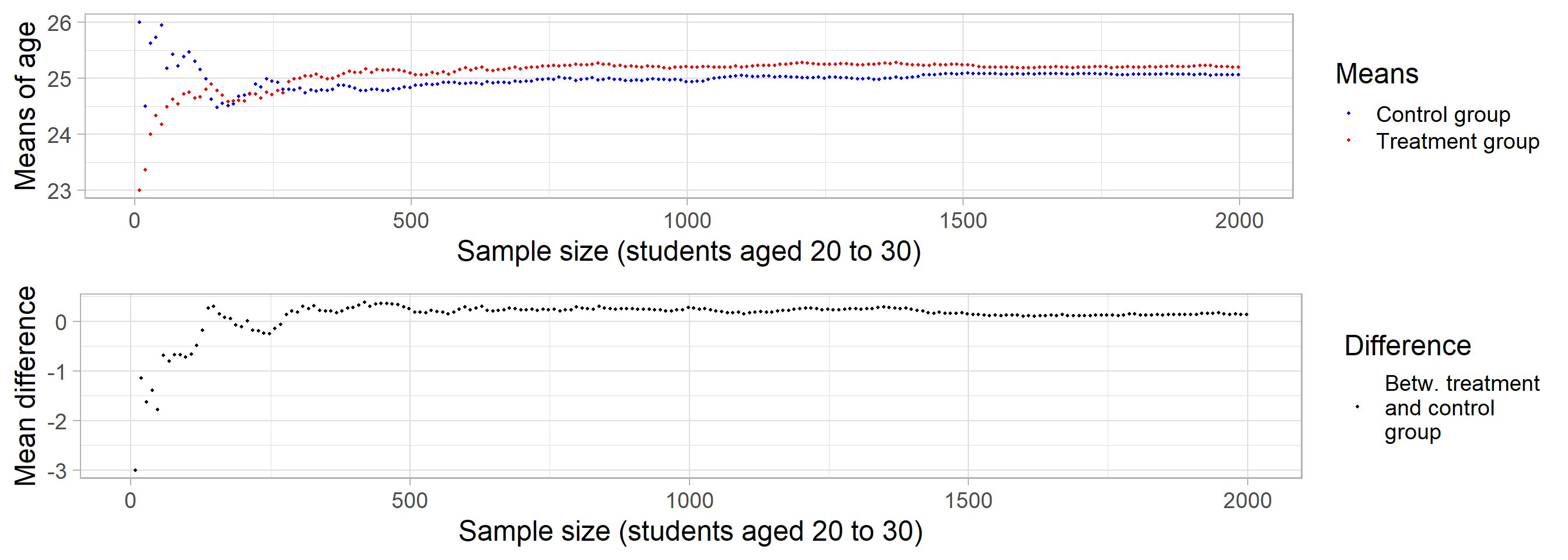
Taxonomy (2): Completely randomized experiments
- Take an even number of units and divide them at random in two groups, with exactly one-half of the sample receiving treatment and remaining receiving control
- e.g., put labels for N units in an urn and draw \(N_{t}=N/2\) and treat them
\[Pr(\mathbf{D}|\mathbf{X},\mathbf{Y}(0),\mathbf{Y}(1)) = \begin{cases} \left( \begin{array}{c} N \\ N_{t} \end{array} \right)^{-1} & \quad \sum_{i=1}^{N} D_{i}=N_{t},\\ 0 & \quad otherwise \end{cases}\]
- Advantage: Treatment/control groups have size we choose (e.g., equal size)
- Disadvantage: Covariates may still be associated with potential outcomes
- Example: Study with N = 20 units, 10 men, 10 women
- Potential treatment and control outcomes vary strongly with sex
- Design assures that 10 get randomly treated but they could be all men (or women)
- Then av. differences would be due to sex rather than treatment
- \(Pr(\mathbf{D}|\mathbf{X},\mathbf{Y}(0),\mathbf{Y}(1))\): Function (assignment mechanism) that assigns probabilities to all possible assignment vectors \(\mathbf{D}\)
\[Pr(\mathbf{D}|\mathbf{X},\mathbf{Y}(0),\mathbf{Y}(1))\] =
\[\begin{cases}\text{Assignment vectors with} \sum_{i=1}^{N} D_{i}=N_{t} \text{occur with probability of} \left(\begin{array}{c}N \\N_{t}\end{array}\right),\\ \text{All other assignment vectors occur with probability} \end{cases}\]
- \(\sum_{i=1}^{N} D_{i}=N_{t}\): Assignment vectors where the sum (= sum of 1s) equals \(N_{t}\) that is the number of treated units
- \(N_{t}\): Number of treated units (does not have to equal \(N/2\))
Completely randomized exp.: Assignment vectors
- Q: With \(N = 4\) and \(N_{t} = 2\) we have 6 possible assignment vectors. Which one(s) would you prefer? What is the probability of one of them occuring?
| unit | D1 | D2 | D3 | D4 | D5 | D6 |
|---|---|---|---|---|---|---|
| Simon | 1 | 1 | 0 | 1 | 0 | 0 |
| Julia | 1 | 0 | 1 | 0 | 1 | 0 |
| Claudia | 0 | 1 | 1 | 0 | 0 | 1 |
| Diego | 0 | 0 | 0 | 1 | 1 | 1 |
\(\left(\begin{array}{c}N \\ N_{t}\end{array}\right)^{-1}\) = \(\left(\frac{N!}{N_{t}!\,(N-N_{t})!}\right)^{-1}\) = \(\left(\begin{array}{c}4\\ 2\end{array}\right)^{-1}\) = \(\left(\frac{4!}{2!\,(4-2)!}\right)^{-1}\) = \(\left(\frac{4\cdot3\cdot2\cdot1}{2\cdot1 \times2\cdot1!}\right)^{-1}\) = \(\left(\frac{24}{4}\right)^{-1}\) = \(\left(6\right)^{-1}\) = \(\frac{1}{6}\)
Q: How many assignment vectors are there if \(N = 4\) and \(N_{t} = 3\)? What is their probability of occuring?
- Yes, 4 assignment vectors and probability 1/4!
- …number of assignment vectors is reduced as compared to Bernoulli trial!
Taxonomy (3): Stratified randomized experiments
Population of units in the study is first partitioned into blocks or strata
- Units within each block similar with respect to some (functions of) covariates thought to be predictive of potential outcomes
Within each block, we conduct a completely randomized experiment, with assignments independent across blocks
Example: 2 blocks, e.g., males and females, where independent completely randomized (block) experiments are conducted for each group/block
Assignment mechanism (see Imbens and Rubin 2015, 52): Same formula as completely randomized experiments but replacing \(N\) and \(N_{t}\) with \(N(m)\) and \(N_{t}(m)\) for males and \(N(f)\) and \(N_{t}(f)\) for females
Taxonomy (4): Paired randomized experiments
- Also called paired comparison or randomized paired design
- Extreme version of the randomized block experiment in which there are exactly two units within each block
- Fair coin is tossed to decide which unit in pair gets treatment
- See Imbens and Rubin (2015, 53) for assignment mechanism function
- Example: Educational experiment with covariate pre-test score
- You would be ranked from high to low
- Top two = 1st pair
- Next two = 2nd pair
- Next two = …
- Within each pair one unit is assigned to treatment with probability 1/2
Exercise: Assignment & randomization
Q: What are the main differences between the four types of randomization which we discussed - bernoulli trials, completely randomized experiments; stratified randomized experiments and paired randomized experiments?
Q: Imagine that you conducted an experiment, in which you successfully, randomly assigned participants to treatment and control. What things can still go wrong in a classical randomized experiment?
- Potential issues that might plague experiments
- SUTVA violation; Measurement error; Non-compliance
Appendix F: Parametric statistics (vs. non-parametric)
Branch of statistics which assumes that sample data comes from a population that follows a probability distribution based on a fixed set of parameters (Wikipedia)
- e.g., normal distribution: \(\mathcal{N}\) with \(\mu, \sigma_{2}\)
Since parametric model relies on fixed parameter set, it assumes more about a given population than non-parametric methods
- with correct assumptions it produces more accurate and precise estimates than non-parametric methods
- As more is assumed, when assumptions are not correct it has a greater chance of failing (not a robust stat. method)
Non-parametric model: Parameter set is not fixed, can increase/decrease if new relevant information is collected
Various helpful ressources
Appendix G: Probability
Probability (1)
“Probability” has been defined in different ways
Frequentist view (classical approach)
- Probability as the “frequency of events in a long, perhaps infinite, series of trials” (Lynch 2007, 9)
- “From that perspective, the reason that the probability of achieving a heads on a coin flip is 1/2 is that, in an infinite series of trials, we would see heads 50% of the time” (Ibid, p. 9)
- Most sociologists still follow this paradigm (sometimes not knowing it)
Bayesian view
- Probability as a belief, a “subjective representation of uncertainty about events” (Ibid, p. 9)
- “When we say that the probability of observing heads on a single coin flip is 1/2, we are really making a series of assumptions, including that the coin is fair (i.e., heads and tails are infact equally likely), and that in prior experience or learning we recognize that heads occurs 50% of the time.” (Ibid, p. 9)
Probability distributions (2)
Probability distributions (Everitt 2010, 338) (Examples)
- “a mathematical formula that gives the probability of each value of the variable” (discrete random variable)
- “a curve described by a mathematical formula which specifies, by way of areas under the curve, the probability that the variable falls within a particular interval” (continuous random variable)
- Uni- and multivariate (e.g., multivariate normal, Q: What is the 3rd dimension?)
Also called theoretical distributions (as opposed to empirical distributions of data) and often invented by mathematicians (Q: Most famous one?)
Bernoulli distribution (simplest discrete distribution): e.g., flipping a fair coin
- PMF (Q?) = \(\scriptsize Pr(k) = \begin{cases} q = 1-p & \quad \text{for k} = 0,\\ p & \quad \text{for k} = 1\end{cases}\) (e.g., with p = 0.5)
- Empirical distribution (N = 5), e.g., \(\scriptsize \{0, 1, 1, 0, 1\}\)
- R:
as.numeric(simDAG::rbernoulli(5, 0.5))= 1, 0, 0, 0, 1
Probability distributions (3)
- Q: Why do probability distributions facilitate our work?
- We use probability distributions for statistical inference
- Frequentism/Frequentist inference
- Any given experiment (dataset) can be considered as one of an infinite sequence of possible repetitions of the same experiment
- RQ: What is the average happiness/effect of gender on happiness among Mannheim students?
- Sample of students in class (dataset) = one of infinite sequence of samples we could draw from Mannheim Univ. students
- Sample → Calculate means/mean diff./regression coefficient → Sampling distribution of statistic \(\approx\) probability distribution
- We’ll talk more about uncertainty later on
References
Seminar: Kausalanalyse - Eine Einführung
Abadie, Alberto, Susan Athey, Guido W Imbens, and Jeffrey M Wooldridge. 2020. “Sampling-Based Versus Design-Based Uncertainty in Regression Analysis.” Econometrica 88 (1): 265–96.
Babbie, Earl R. 2015. The Practice of Social Research. Nelson Education.
Bartlett, J W, and C Frost. 2008. “Reliability, Repeatability and Reproducibility: Analysis of Measurement Errors in Continuous Variables.” Ultrasound Obstet. Gynecol. 31 (4): 466–75.
Bauer, Paul C. 2015. “Negative Experiences and Trust: A Causal Analysis of the Effects of Victimization on Generalized Trust.” European Sociological Review 31 (4): 397–417.
Bauer, Paul C, Pablo Barberá, Kathrin Ackermann, and Aaron Venetz. 2017. “Is the Left-Right Scale a Valid Measure of Ideology?” Political Behavior 39 (3): 553–83.
Bauer, Paul C, and Clemm von Hohenberg. 2021. “Believing and Sharing Information by Fake Sources: An Experiment.” Political Communication 38 (6): 647–71.
Bauer, Paul C, and Camille Landesvatter. 2023. “From Ideal Experiments to Ideal Research Designs (IDRs): What They Are and Why We Should Use Them More.”
Cochran, William G. 2007. Sampling Techniques. John Wiley & Sons.
Enos, Ryan D. 2014. “Causal Effect of Intergroup Contact on Exclusionary Attitudes.” Proc. Natl. Acad. Sci. U. S. A. 111 (10): 3699–3704.
Gerring, John. 2012. “Mere Description.” Br. J. Polit. Sci. 42 (4): 721–46.
Holland, Paul W. 1986. “Statistics and Causal Inference.” J. Am. Stat. Assoc. 81 (396): 945–60.
Imai, Kosuke. 2011. “Introduction to the Virtual Issue: Past and Future Research Agenda on Causal Inference.” Political Analysis 19 (V2): 1–4.
Imbens, Guido W, and Donald B Rubin. 2015. Causal Inference for Statistics, Social, and Biomedical Sciences: An Introduction. Cambridge University Press.
Jaccard, James, and Jacob Jacoby. 2019. Theory Construction and Model-Building Skills, Second Edition: A Practical Guide for Social Scientists. Guilford Publications.
Keele, Luke. 2015. “The Discipline of Identification.” PS Polit. Sci. Polit. 48 (01): 102–6.
Moore, Will H, and David A Siegel. 2013. A Mathematics Course for Political and Social Research. Princeton University Press.
Morgan, Stephen L, and Christopher Winship. 2007. Counterfactuals and Causal Inference: Methods and Principles for Social Research. 2 edition. Cambridge University Press.
Open Science Collaboration. 2015. “Estimating the Reproducibility of Psychological Science.” Science 349 (6251): aac4716.
Pearl, Judea. 2009. “Causal Inference in Statistics: An Overview.” Stat. Surv. 3: 96–146.
Pearl, Judea, and Elias Bareinboim. 2014. “External Validity: From Do-Calculus to Transportability Across Populations.” Stat. Sci. 29 (4): 579–95.
Plümper, Thomas. 2014. Effizient Schreiben: Leitfaden Zum Verfassen von Qualifizierungsarbeiten Und Wissenschaftlichen Texten. Walter de Gruyter GmbH & Co KG.
Rubin, Donald B. 1974. “Estimating Causal Effects of Treatments in Randomized and Nonrandomized Studies.” J. Educ. Psychol. 66 (5): 688–701.
Salganik, Matthew J, and Douglas D Heckathorn. 2004. “Sampling and Estimation in Hidden Populations Using Respondent-Driven Sampling.” Sociol. Methodol. 34 (1): 193–240.
Sävje, Fredrik, Michael J Higgins, and Jasjeet S Sekhon. 2017. “Generalized Full Matching and Extrapolation of the Results from a Large-Scale Voter Mobilization Experiment.” arXiv [Stat.ME], March.
———. 2021. “Generalized Full Matching.” Polit. Anal. 29 (4): 423–47.
Sudman, Seymour, and Graham Kalton. 1986. “New Developments in the Sampling of Special Populations.” Annu. Rev. Sociol. 12 (1): 401–29.
Taagepera, Rein. 2008. Making Social Sciences More Scientific: The Need for Predictive Models. OUP Oxford.
Footnotes
Generalizability of a study’s empirical findings to new environments, settings or populations (Pearl and Bareinboim 2014)
Outcome measurement might become a treatment in itself. Make sure that everyone is equally exposed, i.e., that exposure to outcome measurement is constant across units.
Individualistic assignment and SUTVA are both critical assumptions in causal inference but serve different purposes. Individualistic assignment ensures that the treatment assignment for each unit is based solely on its own characteristics, while SUTVA ensures that the potential outcomes for each unit are not influenced by the treatment assignments of other units and that observed outcomes match potential outcomes for the received treatment. Both assumptions help in simplifying the analysis and interpretation of causal effects, but they operate in distinct areas of the causal inference framework. Dependence on Pre-Treatment Variables: Individualistic Assignment focuses on the independence of the treatment assignment probability from the pre-treatment variables of other units. It ensures that the assignment mechanism for each unit is based solely on its own pre-treatment characteristics. SUTVA does not explicitly address the assignment mechanism. Instead, it focuses on the independence of the potential outcomes from the treatment assignments of other units (no interference) and the consistency of observed and potential outcomes. Scope of assumptions: Individualistic Assignment pertains specifically to the mechanism by which treatments are assigned to units, ensuring that this mechanism is individualistic. SUTVA pertains to the nature of potential outcomes and their relationship with treatment assignments, ensuring no interference and consistency. Implications for Analysis: Individualistic Assignment ensures that when modeling the probability of treatment assignment, one needs to consider only the pre-treatment variables of the specific unit. SUTVA ensures that one can interpret potential outcomes meaningfully without worrying about spillover effects from other units’ treatments, simplifying causal inference by focusing on each unit independently.
e.g., \(e(x)=40/(60+40)=0.4\)
Small summary: Same propensity score ≠ Same covariate values; Prop. score matching mimics completeley randomised experiment vs. other matching methods that mimic blocked/stratified randomised experiments