3.7 Two Discrete

3.7.1 Distance Metrics

Some consider distance is not a correlation metric because it isn’t unit independent (i.e., if you scale the distance, the metrics will change), but it’s still a useful proxy. Distance metrics are more likely to be used for similarity measure.

Euclidean Distance
Manhattan Distance
Chessboard Distance
Minkowski Distance
Canberra Distance
Hamming Distance
Cosine Distance
Sum of Absolute Distance
Sum of Squared Distance
Mean-Absolute Error

3.7.2 Statistical Metrics

3.7.2.1 Chi-squared test

3.7.2.1.1 Phi coefficient

2 binary

dt = matrix(c(1,4,3,5), nrow = 2)
dt
#>      [,1] [,2]
#> [1,]    1    3
#> [2,]    4    5
psych::phi(dt)
#> [1] -0.18

3.7.2.1.2 Cramer’s V

between nominal categorical variables (no natural order)

\[ \text{Cramer's V} = \sqrt{\frac{\chi^2/n}{\min(c-1,r-1)}} \]

where

\(\chi^2\) = Chi-square statistic
\(n\) = sample size
\(r\) = # of rows
\(c\) = # of columns

library('lsr')
n = 100 # (sample size)
set.seed(1)
data = data.frame(A = sample(1:5, replace = TRUE, size = n),
                  B = sample(1:6, replace = TRUE, size = n))


cramersV(data$A, data$B)
#> [1] 0.1944616

Alternatively,

ncchisq noncentral Chi-square
nchisqadj Adjusted noncentral Chi-square
fisher Fisher Z transformation
fisheradj bias correction Fisher z transformation

DescTools::CramerV(data, conf.level = 0.95,method = "ncchisqadj")
#>  Cramer V    lwr.ci    upr.ci 
#> 0.3472325 0.3929964 0.4033053

3.7.2.1.3 Tschuprow’s T

2 nominal variables

DescTools::TschuprowT(data)
#> [1] 0.1100808

3.7.3 Ordinal Association (Rank correlation)

Good with non-linear relationship

3.7.3.1 Ordinal and Nominal

n = 100 # (sample size)
set.seed(1)
dt = table(data.frame(
    A = sample(1:4, replace = TRUE, size = n), # ordinal
    B = sample(1:3, replace = TRUE, size = n)  # nominal
)) 
dt
#>    B
#> A    1  2  3
#>   1  7 11  9
#>   2 11  6 14
#>   3  7 11  4
#>   4  6  4 10

3.7.3.1.1 Freeman’s Theta

Ordinal and nominal

# this package is not available for R >= 4.0.0
rcompanion::freemanTheta(dt, group = "column") 
# because column is the grouping variable (i.e., nominal)

3.7.3.1.2 Epsilon-squared

Ordinal and nominal

# this package is not available for R >= 4.0.0
rcompanion::epsilonSquared(dt,group = "column" ) 
# because column is the grouping variable (i.e., nominal)

3.7.3.2 Two Ordinal

n = 100 # (sample size)
set.seed(1)
dt = table(data.frame(
    A = sample(1:4, replace = TRUE, size = n), # ordinal
    B = sample(1:3, replace = TRUE, size = n)  # ordinal
)) 
dt
#>    B
#> A    1  2  3
#>   1  7 11  9
#>   2 11  6 14
#>   3  7 11  4
#>   4  6  4 10

3.7.3.2.1 Goodman Kruskal’s Gamma

2 ordinal variables

DescTools::GoodmanKruskalGamma(dt, conf.level = 0.95)
#>        gamma       lwr.ci       upr.ci 
#>  0.006781013 -0.229032069  0.242594095

3.7.3.2.2 Somers’ D

or Somers’ Delta
2 ordinal variables

DescTools::SomersDelta(dt, conf.level = 0.95)
#>       somers       lwr.ci       upr.ci 
#>  0.005115859 -0.172800185  0.183031903

3.7.3.2.3 Kendall’s Tau-b

2 ordinal variables

DescTools::KendallTauB(dt, conf.level = 0.95)
#>        tau_b       lwr.ci       upr.ci 
#>  0.004839732 -0.163472443  0.173151906

3.7.3.2.4 Yule’s Q and Y

2 ordinal variables

Special version \((2 \times 2)\) of the Goodman Kruskal’s Gamma coefficient.

	Variable 1
Variable 2	a	b
	c	d

\[ \text{Yule's Q} = \frac{ad - bc}{ad + bc} \]

We typically use Yule’s \(Q\) in practice while Yule’s Y has the following relationship with \(Q\).

\[ \text{Yule's Y} = \frac{\sqrt{ad} - \sqrt{bc}}{\sqrt{ad} + \sqrt{bc}} \]

\[ Q = \frac{2Y}{1 + Y^2} \]

\[ Y = \frac{1 = \sqrt{1-Q^2}}{Q} \]

n = 100 # (sample size)
set.seed(1)
dt = table(data.frame(A = sample(c(0, 1), replace = TRUE, size = n),
                  B = sample(c(0, 1), replace = TRUE, size = n)))
dt
#>    B
#> A    0  1
#>   0 25 24
#>   1 28 23

DescTools::YuleQ(dt)
#> [1] -0.07778669

3.7.3.2.5 Tetrachoric Correlation

is a special case of Polychoric Correlation when both variables are binary

library(psych)

n = 100 # (sample size)

data = data.frame(A = sample(c(0, 1), replace = TRUE, size = n),
                  B = sample(c(0, 1), replace = TRUE, size = n))

#view table
head(data)
#>   A B
#> 1 1 0
#> 2 1 0
#> 3 0 0
#> 4 1 0
#> 5 1 0
#> 6 1 0

table(data)
#>    B
#> A    0  1
#>   0 21 23
#>   1 34 22


#calculate tetrachoric correlation
tetrachoric(data)
#> Call: tetrachoric(x = data)
#> tetrachoric correlation 
#>   A    B   
#> A  1.0     
#> B -0.2  1.0
#> 
#>  with tau of 
#>     A     B 
#> -0.15  0.13

3.7.3.2.6 Polychoric Correlation

between ordinal categorical variables (natural order).
Assumption: Ordinal variable is a discrete representation of a latent normally distributed continuous variable. (Income = low, normal, high).

library(polycor)

n = 100 # (sample size)

data = data.frame(A = sample(1:4, replace = TRUE, size = n),
                  B = sample(1:6, replace = TRUE, size = n))

head(data)
#>   A B
#> 1 1 3
#> 2 1 1
#> 3 3 5
#> 4 2 3
#> 5 3 5
#> 6 4 4


#calculate polychoric correlation between ratings
polychor(data$A, data$B)
#> [1] 0.01607982

3.7.4 Summary

library(tidyverse)

data("mtcars")
df = mtcars %>%
    dplyr::select(cyl, vs, carb)


df_factor = df %>%
    dplyr::mutate(
        cyl = factor(cyl),
        vs = factor(vs),
        carb = factor(carb)
    )
# summary(df)
str(df)
#> 'data.frame':    32 obs. of  3 variables:
#>  $ cyl : num  6 6 4 6 8 6 8 4 4 6 ...
#>  $ vs  : num  0 0 1 1 0 1 0 1 1 1 ...
#>  $ carb: num  4 4 1 1 2 1 4 2 2 4 ...
str(df_factor)
#> 'data.frame':    32 obs. of  3 variables:
#>  $ cyl : Factor w/ 3 levels "4","6","8": 2 2 1 2 3 2 3 1 1 2 ...
#>  $ vs  : Factor w/ 2 levels "0","1": 1 1 2 2 1 2 1 2 2 2 ...
#>  $ carb: Factor w/ 6 levels "1","2","3","4",..: 4 4 1 1 2 1 4 2 2 4 ...

Get the correlation table for continuous variables only

cor(df)
#>             cyl         vs       carb
#> cyl   1.0000000 -0.8108118  0.5269883
#> vs   -0.8108118  1.0000000 -0.5696071
#> carb  0.5269883 -0.5696071  1.0000000

# only complete obs
# cor(df, use = "complete.obs")

Alternatively, you can also have the

Hmisc::rcorr(as.matrix(df), type = "pearson")
#>        cyl    vs  carb
#> cyl   1.00 -0.81  0.53
#> vs   -0.81  1.00 -0.57
#> carb  0.53 -0.57  1.00
#> 
#> n= 32 
#> 
#> 
#> P
#>      cyl    vs     carb  
#> cyl         0.0000 0.0019
#> vs   0.0000        0.0007
#> carb 0.0019 0.0007

modelsummary::datasummary_correlation(df)

	cyl	vs	carb
cyl	1	.	.
vs	−.81	1	.
carb	.53	−.57	1

ggcorrplot::ggcorrplot(cor(df))

Different comparison between different correlation between different types of variables (i.e., continuous vs. categorical) can be problematic. Moreover, the problem of detecting non-linear vs. linear relationship/correlation is another one. Hence, a solution is that using mutual information from information theory (i.e., knowing one variable can reduce uncertainty about the other).

To implement mutual information, we have the following approximations

\[ \downarrow \text{prediction error} \approx \downarrow \text{uncertainty} \approx \downarrow \text{association strength} \]

More specifically, following the X2Y metric, we have the following steps:

Predict \(y\) without \(x\) (i.e., baseline model)
1. Average of \(y\) when \(y\) is continuous
2. Most frequent value when \(y\) is categorical
Predict \(y\) with \(x\) (e.g., linear, random forest, etc.)
Calculate the prediction error difference between 1 and 2

To have a comprehensive table that could handle

continuous vs. continuous
categorical vs. continuous
continuous vs. categorical
categorical vs. categorical

the suggested model would be Classification and Regression Trees (CART). But we can certainly use other models as well.

The downfall of this method is that you might suffer

Symmetry: \((x,y) \neq (y,x)\)
Comparability : Different pair of comparison might use different metrics (e.g., misclassification error vs. MAE)

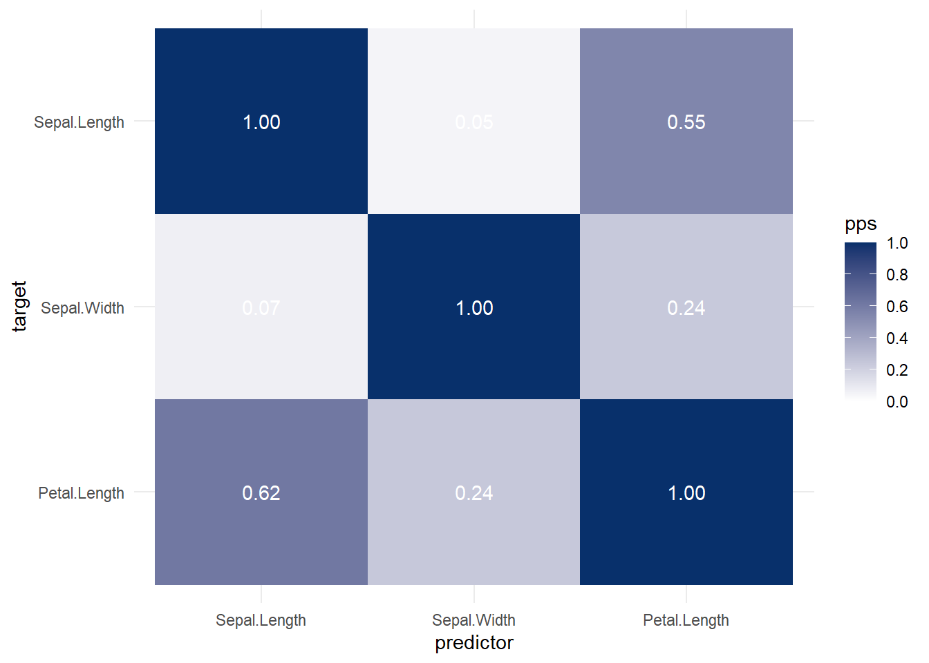
library(ppsr)

iris <- iris %>% 
  select(1:3)

# ppsr::score_df(iris) # if you want a dataframe
ppsr::score_matrix(iris,
                   do_parallel = TRUE,
                   n_cores = parallel::detectCores() / 2)
#>              Sepal.Length Sepal.Width Petal.Length
#> Sepal.Length   1.00000000  0.04632352    0.5491398
#> Sepal.Width    0.06790301  1.00000000    0.2376991
#> Petal.Length   0.61608360  0.24263851    1.0000000

# if you want a similar correlation matrix
ppsr::score_matrix(df,
                   do_parallel = TRUE,
                   n_cores = parallel::detectCores() / 2)
#>             cyl        vs      carb
#> cyl  1.00000000 0.3982789 0.2092533
#> vs   0.02514286 1.0000000 0.2000000
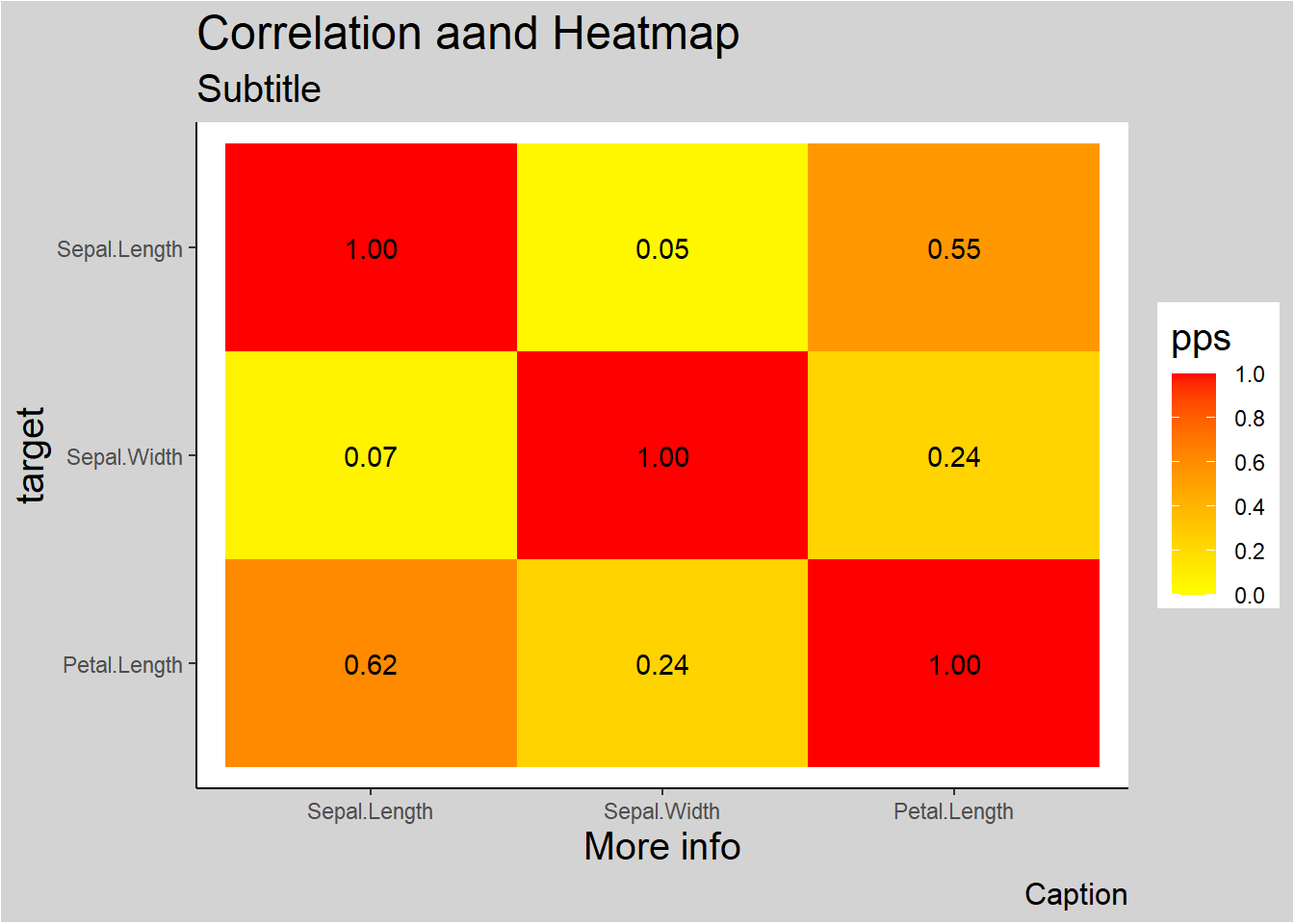
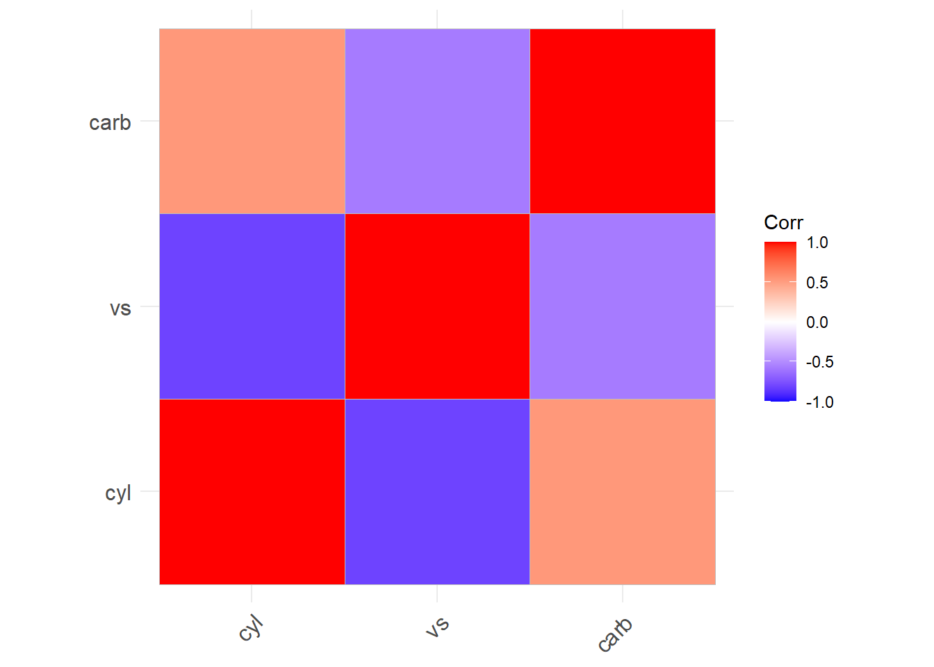
#> carb 0.30798148 0.2537309 1.0000000

3.7.5 Visualization

corrplot::corrplot(cor(df))

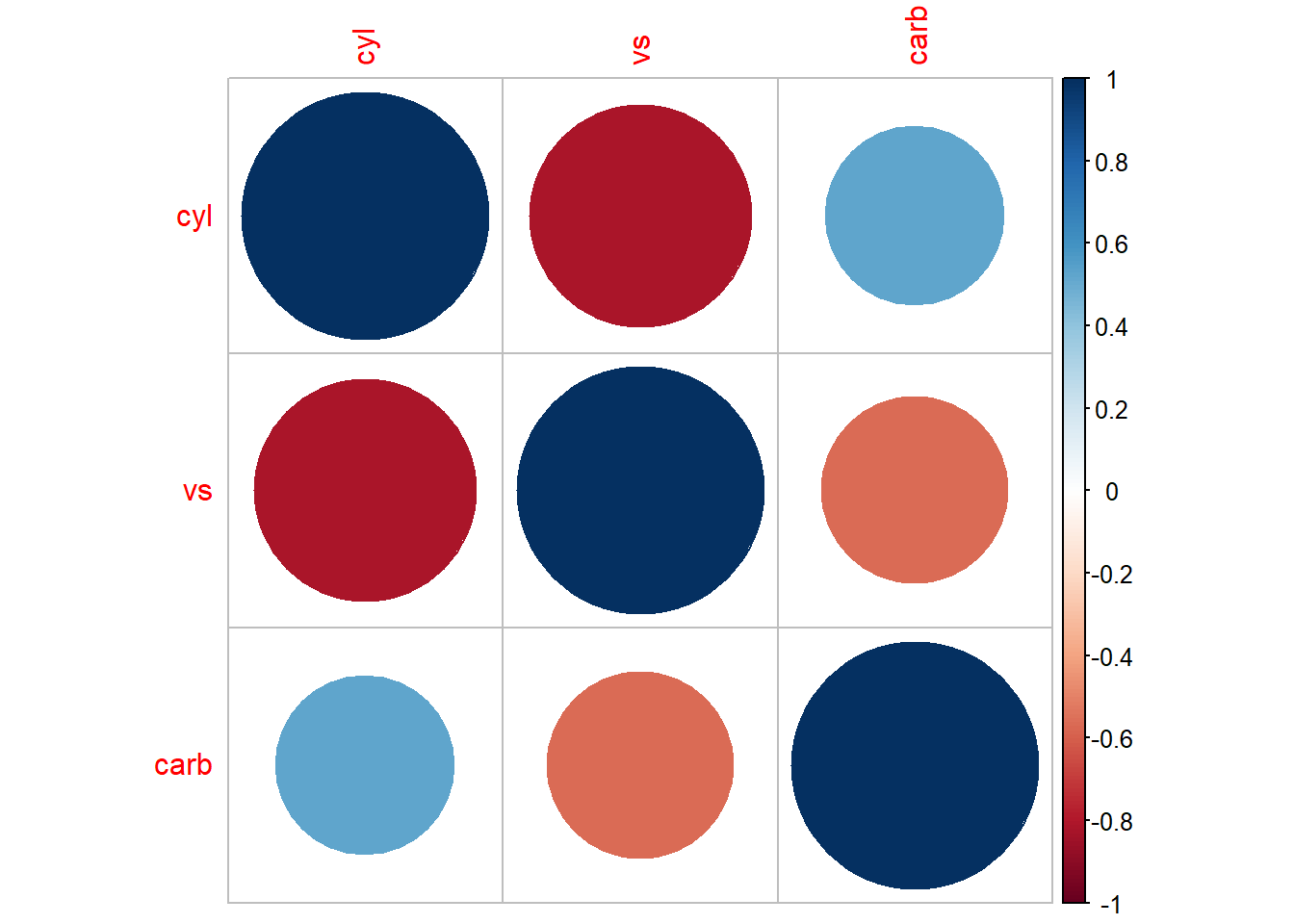
Alternatively,

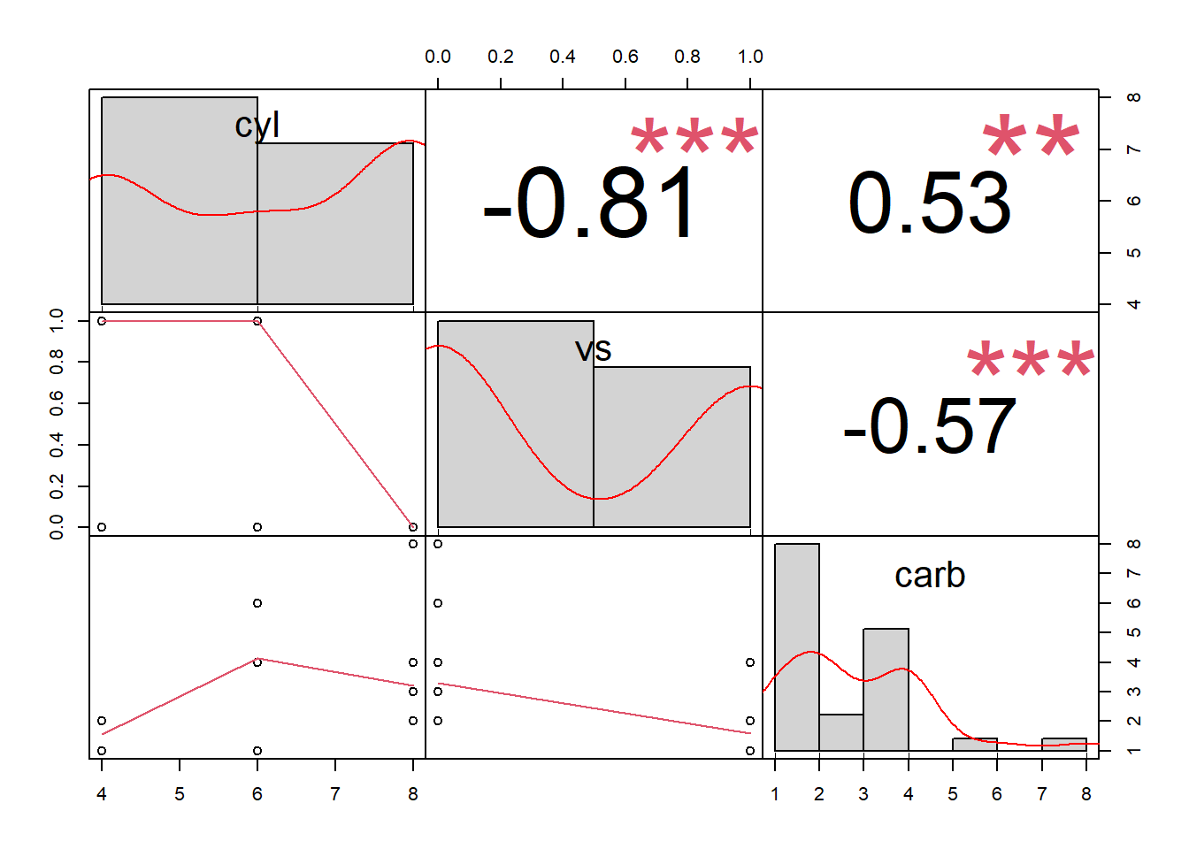
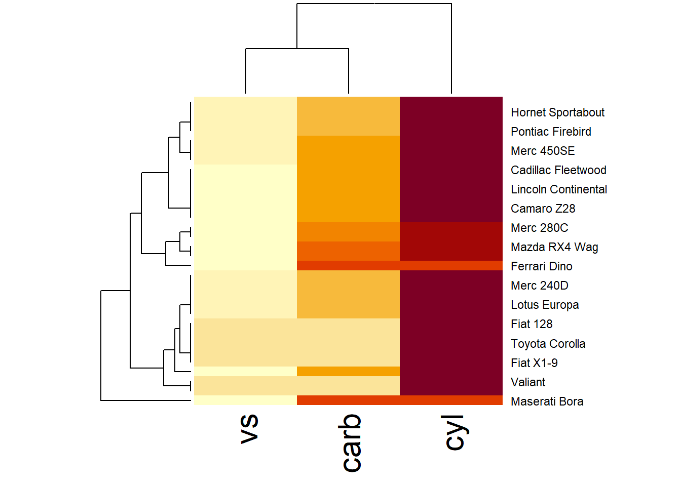
PerformanceAnalytics::chart.Correlation(df, histogram = T, pch = 19)

heatmap(as.matrix(df))

More general form,

ppsr::visualize_pps(
    df = iris,
    do_parallel = TRUE,
    n_cores = parallel::detectCores() / 2
)

ppsr::visualize_correlations(
    df = iris
)

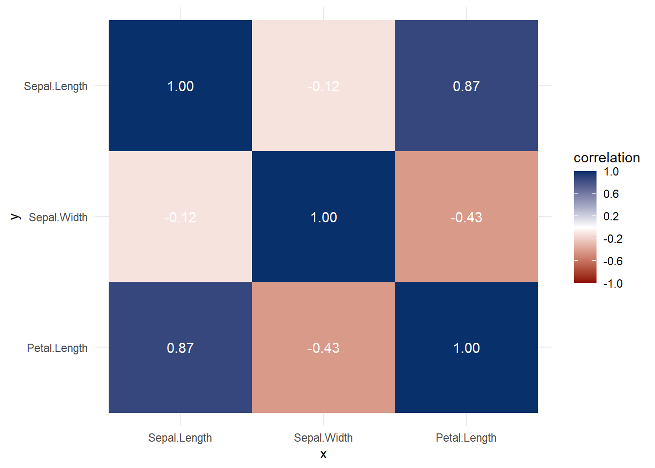
Both heat map and correlation at the same time

ppsr::visualize_both(
    df = iris,
    do_parallel = TRUE,
    n_cores = parallel::detectCores() / 2
)

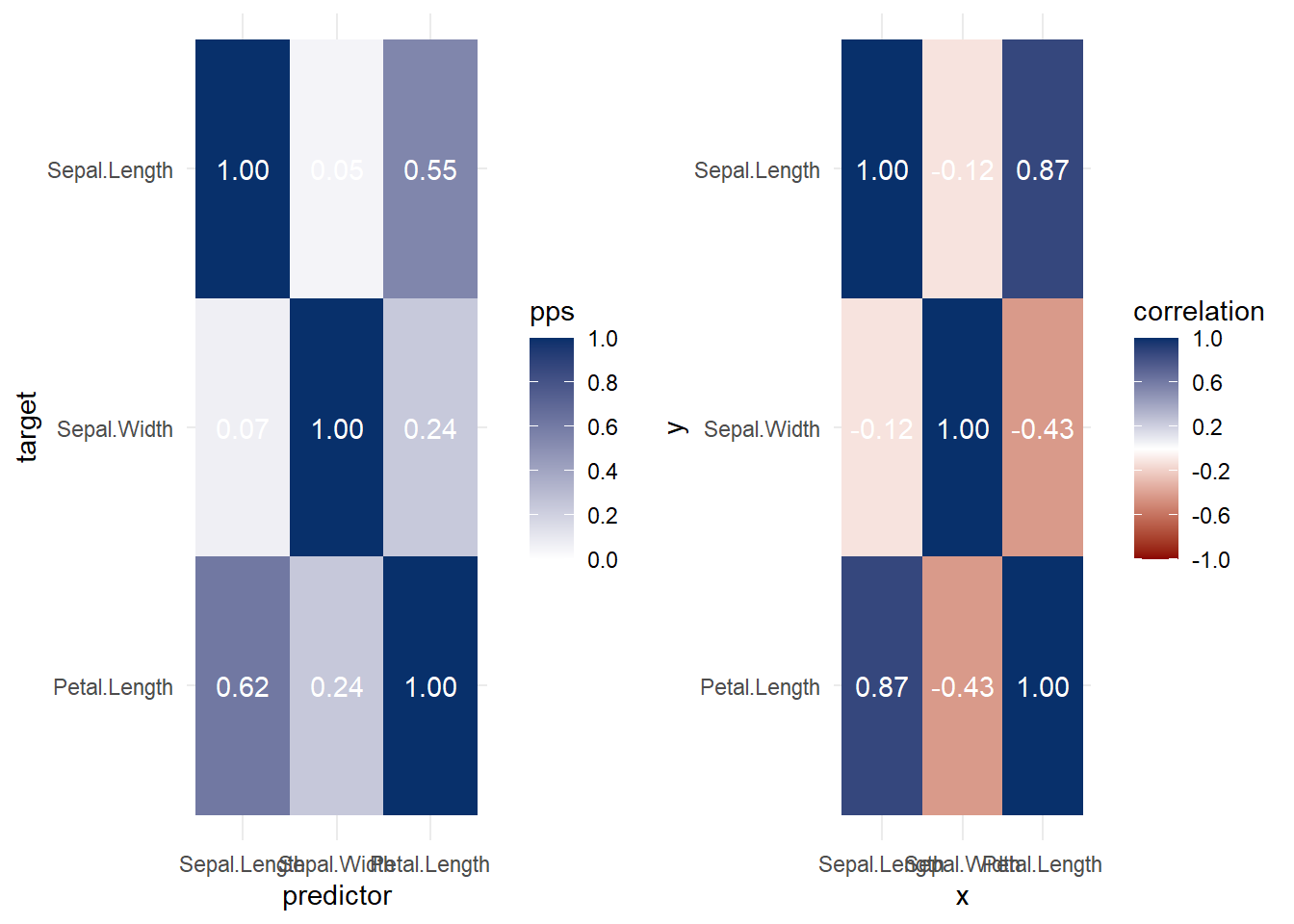
More elaboration with ggplot2

ppsr::visualize_pps(
    df = iris,
    color_value_high = 'red',
    color_value_low = 'yellow',
    color_text = 'black'
) +
    ggplot2::theme_classic() +
    ggplot2::theme(plot.background = 
                       ggplot2::element_rect(fill = "lightgrey")) +
    ggplot2::theme(title = ggplot2::element_text(size = 15)) +
    ggplot2::labs(
        title = 'Correlation aand Heatmap',
        subtitle = 'Subtitle',
        caption = 'Caption',
        x = 'More info'
    )