Chapter 9 Location Allocations
9.1 Setup: Packages and Data
You will need to load the following packages, testing for the presence on your R installation as before (although in a different way!):
packages <- c("sf", "tidyverse","tmap", "devtools", "gtools")
# check which packages are not installed
not_installed <- packages[!packages %in% installed.packages()[, "Package"]]
# install missing packages
if (length(not_installed) > 1) {
  install.packages(not_installed, repos = "https://cran.rstudio.com/", dep = T)
}
# load the packages
library(sf)         # for spatial data
library(tidyverse)  # for data wrangling
library(tmap)       # for mapping
library(devtools)
library(gtools)
We also need the tbart package and this needs to be installed in a different way using the install_version function of the devtools package and the load the package with the library function.
install_version("tbart", version = "1.0", dep = T)library(tbart)And you will need to load the georgia data as in previous practicals.
download.file("https://github.com/gwverse/gw/blob/main/data/georgia.rda?raw=True",
              "./georgia.RData", mode = "wb")
load("georgia.RData")
You should examine this in the usual way:
# spatial data
georgia
summary(georgia)
tm_shape(georgia) + tm_borders()
tm_shape(georgia) + tm_polygons("MedInc")
You will also need some data from the VLE for later sections:
wz = st_read("Trafford_WPZsPop.gpkg", quiet = T) %>% `st_crs<-`(27700)## Warning: st_crs<- : replacing crs does not reproject data; use st_transform for
## thatstores = read.csv("geog3191grocers2016.csv")9.2 Location allocation overview
Location allocation is a suite of techniques for determining optimal facility siting and locations relative to some measure of spatial demand. It can be used in a number of ways:
- to determine locations for new facilities (shops, hospitals, etc).
- to reorganise or reallocate existing facilities (in order to better service the demand for them).
- to determine which facilities to close based on a set of spatial constraints.
In this sense location allocation relates to supply and demand. What it seeks to do is to identify the locations that best satisfy spatially distributed demand.
Supply can be considered as the provision of facilities at specific locations, either current or future. Often the resources need to supply the demands at any given location are assumed to exist - nurses needed for a hospital, deliveries for a shop, but they also involve some weighting based on supply capacity of some kind, for example floor area as is used in retail geography.
Demand maybe conceived as a simple distance or other cost (financial or travel time for example) and may be weighted maybe by some measure of targeted demand. these may be simple counts of population, or targeted subgroups such existing customers, people with disabilities, children, unemployed etc.
There are a number of important and related considerations in location allocation modelling:
1. The problem of dimensionality In only very few cases is it possible to identify the best set of locations deterministically. That is, by evaluating each set of possible solutions. This is because of the extremely large number of possible sets of solutions to even very small problems. Consider the problem of identifying the best 25 locations from 10000 possible locations (for example locations spaced at 100m in a 10km x 10km study area). The number of different combinations facilities to evaluate is very large:
\[\frac{10000! }{ (25! \times (10000!-25!)}\]
This equals \(4.15e+35684\) permutations of solutions to evaluate. This is impossible to deterministically (i.e. one by one).
2. Searching through the space The dimensionality problem means that all possible sets of solutions cannot be individually evaluated. This is because the search space the number of possible solutions is too great. To overcome this what are called heuristic searches or search heuristics are used to search through the solution space. These look for local optima and try to determine whether these are globally optimal as well. Different approaches tackle this search in different ways. the basic idea is that they find parts of the solution space that are quite good and try to search deeper within these in different ways. These include things you may have heard of such as genetic algorithms, tabu searches. One such approach is the Teitz and Bart heuristic which is used in the examples in this practical.
3. Optimality and the evaluation function Location allocation seeks to determine the best or optimal set of locations for facility given demand. In order to determine the optimal set of facility locations given some spatial distribution of demand, requires that what is meant by best or optimal is defined in some way. This is done through an evaluation function which helps the heuristic search through the solution space. A common objective is, for example, to minimise demand weighted distance to a set of facilities. The evaluation function controls the heuristic search - it determines what is “good” and therefore defines the regions in the solution space that are examined more deeply.
4. Demand Weighting The evaluation function can evaluate just distances (e.g. to the nearest facility) for each demand location, or these can be weighted in some way. Weights might reflect customers, segments of the population, or other characteristics of the demand areas, such as deprivation. Many location allocation analyses seek to minimise measures such as demand weighted distance, measured in units such as person kilometres. It is a concept assumes that facility access and distances are important but the weights could be other things such as spending power. The worked example below demonstrates this.
Worked Example Consider the matrix of distances between demand locations, A, B and C and potential supply locations 1,2,3 and 4 in the table below.
# define a distance matrix
A = c(10, 190, 180, 150)
B = c(180, 10, 120, 150)
C = c(150, 150, 10, 150)
df = t(data.frame(A = A,B = B,C=C))
colnames(df) = c(1:4)
# have a look
df
## 1 2 3 4
## A 10 190 180 150
## B 180 10 120 150
## C 150 150 10 150If we wanted to identify the best 2 locations based distance alone, then we would evaluates each set of 2 supply locations and find the set that minimises the distance of each demand location to its nearest supply location. The combinations function is useful in this very simple case. It is used below to create an object, gr, of all possible sets of locations:
gr = combinations(n=4, r =2, v= c(1:4))
gr
## [,1] [,2]
## [1,] 1 2
## [2,] 1 3
## [3,] 1 4
## [4,] 2 3
## [5,] 2 4
## [6,] 3 4We can use this to evaluated the simple distance based case. The loop below takes each set of potential locations and evaluates the distance of each demand location to the nearest supply. The results show that locations 1 and 3 provide the optimal set of locations, when “optimal” is defined on distance alone.
res.out = vector()
for (i in 1:nrow(gr)) {
  # select the potential locations
  index = unlist(gr[i,])
  # get their distances
  df.i = df[, index]
  # extract the min distance for each row (demand)
  res.i = sum(apply(df.i, 1, min))
  # add the result to the result vector
  res.out = append(res.out, res.i)
}
cbind(gr, res.out)
## res.out
## [1,] 1 2 170
## [2,] 1 3 140
## [3,] 1 4 310
## [4,] 2 3 200
## [5,] 2 4 310
## [6,] 3 4 280We can add some demand weighting:
df2 = data.frame(df, Pop = c(100, 250, 350))
df2
## X1 X2 X3 X4 Pop
## A 10 190 180 150 100
## B 180 10 120 150 250
## C 150 150 10 150 350And use this in our evaluation of each set. This time the evaluation of each candidate location in each set incorporates distance weighted by demand population, resulting a different set of locations being identified as optimal, locations 2 and 3:
res.out = vector()
for (i in 1:nrow(gr)) {
  # select the potential locations
  index = unlist(gr[i,])
  # get their distances
  df.i = df2[, index]
  # extract the min distance for each row (demand) * Pop
  res.i = sum(apply(df.i, 1, min) * df2$Pop)
  # add the result to the result vector
  res.out = append(res.out, res.i)
}
cbind(gr, res.out)
## res.out
## [1,] 1 2 56000
## [2,] 1 3 34500
## [3,] 1 4 91000
## [4,] 2 3 24000
## [5,] 2 4 70000
## [6,] 3 4 48500However this deterministic approach although transparent, will not work with many everyday problems and applications. The next sections provide two case studies based on published work, that are more complex and thus dimensional that this simple example.
9.2.1 Summary
- The aim of location allocation is to optimise the siting of \(n\) facilities given a set of potential locations.
- it is important to note that sets of potential solutions are evaluated together rather identifying the best location, then the next best and so on.
- The computational space can easily be very large and all effective algorithms use some kind of heuristic search to identify the \(n\) best locations.
- Typically approaches use algorithms that seek to minimise some kind of demand weighted distance (e.g. with units such as person kilometres). This results in the locations that are the most easily accessed by the most people being selected.
9.3 Allocation with the tbart package
The tbart package provides an implementation of Teitz and Bart’s algorithm. This attempts to find subset of size \(p\) within a set of potential supply points such that summed distances of the demand locations (also points) in the set allocated to the nearest supply point in \(p\) is minimised. The package notes that “Although generally effective, this algorithm does not guarantee that a globally optimal subset is found”.
The tbart package hasn’t yet been updated to work with sf format objects and so spatial data needs to be converted to sp format. The code below uses the Georgia data sp format so the data iinsf` format need to be converted. What the code below below does is to determine the best 5 counties out of 159 to site some kind of facility in order to best cover the demands represented by the counties. In this first example there is no weighting by population etc, it is purely evaluated on distance.
# convert georgia to sp
georgia_sp = as(georgia, "Spatial")

# find the best 5 counties to allocate others to
set.seed(123)
allocations.list <- allocate(georgia_sp, p=5)

# merge the counties allocated to each point
# this function does this - run all in one go to compile it
st_union_by = function(geo, group) {
  y2 = vector()
  count = 1
  #loop over by groups and merge units
  for (i in unique(group)) {
    #which units
    z = geo[which(group == i),]
    #merge
    y = (st_union(z))
    y2 = rbind(y2, y)
    #y2[[count]] = y
    count = count + 1
  }
  # create the output
  out = st_sfc((y2))
  # set the crs
  st_crs(out) = st_crs(geo)
  # return
  out
}
# and then call it to create the zones object
zones = st_union_by(georgia, allocations.list)
# plot the result
tm_shape(georgia) + tm_polygons() +
  tm_shape(zones) + tm_borders(col = "red", lty = 2, lwd = 3) +
  tm_shape(georgia[unique(allocations.list), ]) + tm_polygons("red")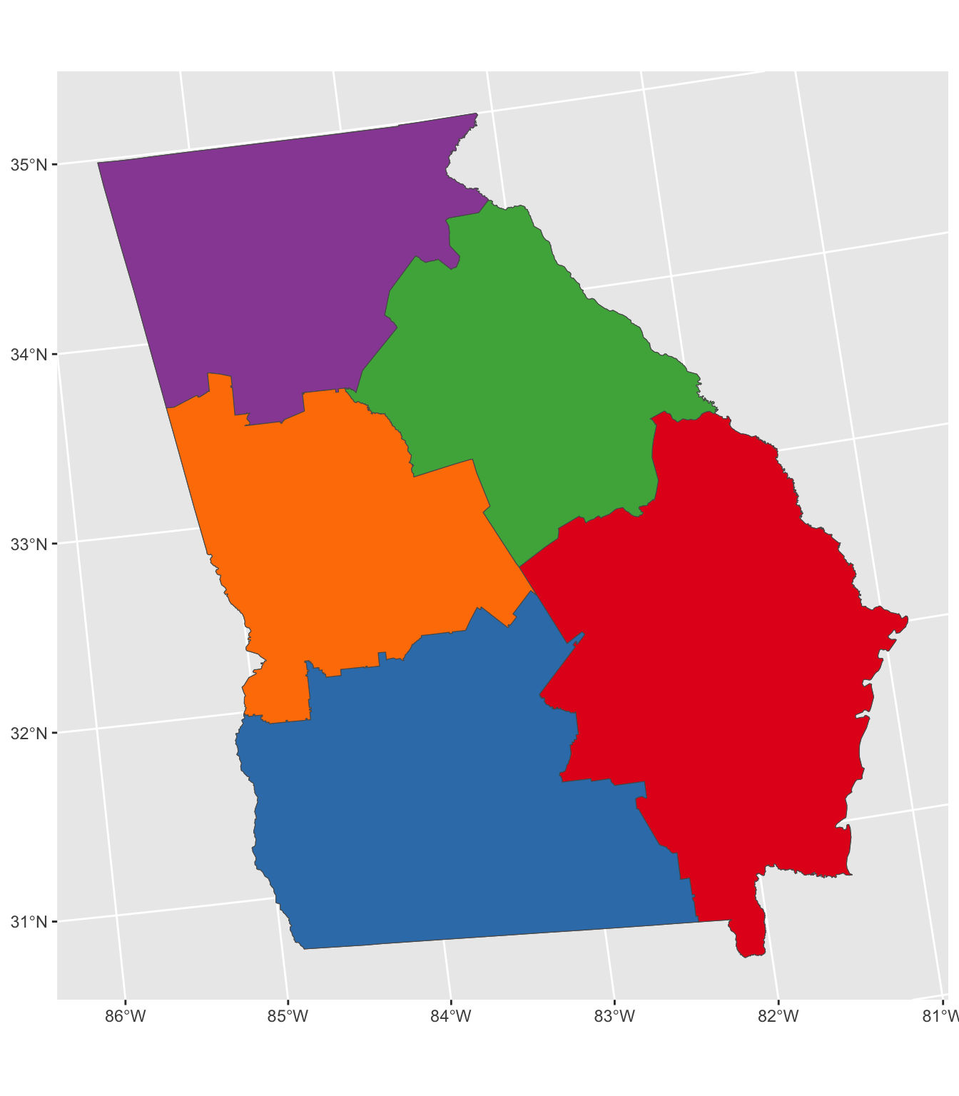
Figure 9.1: Allocation without weights.
What this has done is take the counties, convert them into points (their geometric centroids) and use these as both the supply and demand locations. If a distance matrix of the distances between supply and demand locations is not supplied then the allocate function calculates it.
In the code below the distance matrix is pre calculated and is weighted by population using the attributes in the Georgia data set before being passed to the allocate function.
# convert georgia to pints (not needed but is more transparent)
georgia_pt = st_centroid(georgia)
## Warning in st_centroid.sf(georgia): st_centroid assumes attributes are constant
## over geometries of x# distance matrix
dmat = st_distance(georgia_pt, georgia_pt)
dmat[1:6, 1:6]## Units: [m]
## [,1] [,2] [,3] [,4] [,5] [,6]
## [1,] 0.00 75237.10 26712.93 209277.4 172409.6 311599.8
## [2,] 75237.10 0.00 49540.34 148426.6 200462.4 345831.5
## [3,] 26712.93 49540.34 0.00 190341.1 184671.5 327228.2
## [4,] 209277.45 148426.65 190341.07 0.0 224285.0 349132.7
## [5,] 172409.59 200462.42 184671.54 224285.0 0.0 145384.7
## [6,] 311599.80 345831.51 327228.18 349132.7 145384.7 0.0# weight dmat by pop
dmatw = dmat*georgia_pt$TotPop90You can check that this has done what it should: consider the rows in dmat as the demand locations and the columns as potential supply points. In the first row of the weighted distance matrix (i.e. demand weighted distance), we would expect the distances to be multiplied by the population of the first county (15744):
# check 1st row first 6 population values
head(georgia_pt$TotPop90)
## [1] 15744 6213 9566 3615 39530 10308# check 1st row first 6 columns of dmat
dmat[1, 1:6]## Units: [m]
## [1] 0.00 75237.10 26712.93 209277.45 172409.59 311599.80# check 1st row first 6 columns times 1st pop value
dmat[1, 1:6] * 15744## Units: [m]
## [1] 0 1184532840 420568432 3294864129 2714416565 4905827189# check 1st row first 6 columns of weighted dmat
dmatw[1, 1:6]## Units: [m]
## [1] 0 1184532840 420568432 3294864129 2714416565 4905827189We can now plug this weighted distance matrix into the allocation and this pulls the allocations towards the large centres of population:
set.seed(120)
allocations.list <- allocate(georgia_sp, metric = dmatw, p=5)
zones = st_union_by(georgia, allocations.list)
# plot the results
# plot the result
tm_shape(georgia) + tm_polygons() +
  tm_shape(zones) + tm_borders(col = "red", lty = 2, lwd = 3) +
  tm_shape(georgia[unique(allocations.list), ]) + tm_polygons("red")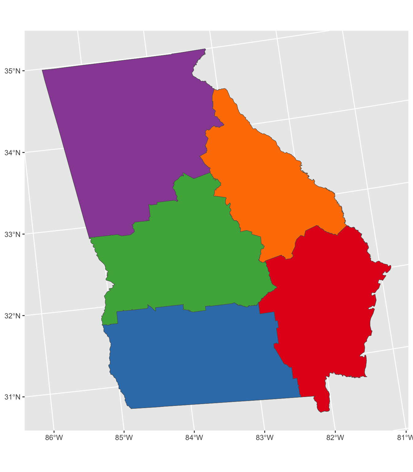
Figure 9.2: Allocation with weights.
Finally, we can plot the allocations using a star diagram. The function below creates this from the outputs of the allocations function using the outputs of the allocate function and converting them to sf format. This generates the lines representation of the allocations.
# create allocations
georgia_allocs <- allocations(georgia_sp,p=5,force=unique(allocations.list))
# convert to sf
georgia_allocs = st_as_sf(georgia_allocs)
# create star lines function
create_star_lines = function (sf1,sf2, alloc) {
    if (missing(sf2))
        sf2 <- sf1
    if (missing(alloc)) {
        alloc <- sf1$allocation
    }
    co1 <- st_coordinates(st_centroid(sf1))
    co2 <- st_coordinates(st_centroid(sf2))
    result <- matrix(nrow = 0, ncol = 5)
    for (i in 1:nrow(co1)) {
      result <- rbind(result,  c(i, c(co1[i, 1], co2[alloc[i], 1]), c(co1[i, 2], co2[alloc[i], 2]) ) )
    }
    result = as.data.frame(result)
    ls <- apply(result, 1, function(x)
      {
      v <- as.numeric(x[c(2,3,4,5)])
      m <- matrix(v, nrow = 2)
      return(st_sfc(st_linestring(m), crs = st_crs(sf1)))
      })
    ls = Reduce(c, ls)
    star_lines = data.frame(ID = result$V1)
    st_geometry(star_lines) = ls
    return(star_lines)
}
star_lines <- create_star_lines(georgia_allocs)
## Warning in st_centroid.sf(sf1): st_centroid assumes attributes are constant over
## geometries of x## Warning in st_centroid.sf(sf2): st_centroid assumes attributes are constant over
## geometries of xAnd the results can be mapped as in Figure 9.3.
# star lines
p1 = tm_shape(georgia) + tm_borders(col = "lightgrey") +
  tm_shape(star_lines)+tm_lines(col = "darkred", lwd = 2)
# distance to allocation
p2 = tm_shape(georgia_allocs) +
  tm_polygons(col = "allocdist",
              title = "Distance",
              palette = "Reds", n = 7, style = "kmeans")
tmap_arrange(p1, p2)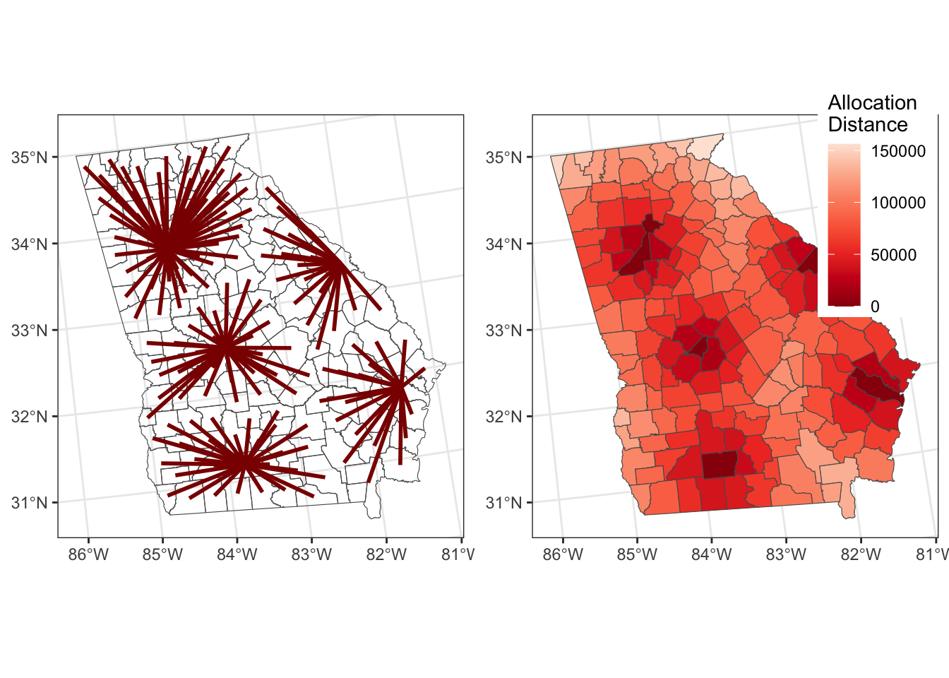
Figure 9.3: The results of the allocations, showing the allocation lines and distances.
9.4 Location-Allocation for supply and demand modelling
The previous section determined the locations that minimised either weighted or unweighed distance between each area to a single location.
In this section a more realistic application is developed: where to locate a new convenience store. Our objective it to identify potential locations for 3 new new convenience stores. We have some data from GEOG3191 of existing grocery stores in the Trafford area of Manchester and some indication of demand through a workplace zone population, which we can use as our target population.
It is instructive to have a quick look at the data you loaded earlier. Figure 9.4 shows the workplace zones and the the head of the stores data:
# full map with embellishments
tm_shape(wz) + tm_polygons("TotalWP", palette = "YlOrRd", n = 10, type = "kmeans") +
  tm_layout(legend.position = c("left", "top")) +
    tm_compass(type = "rose", position = c("left", "bottom")) +
tm_scale_bar(position = c("left", "bottom")) 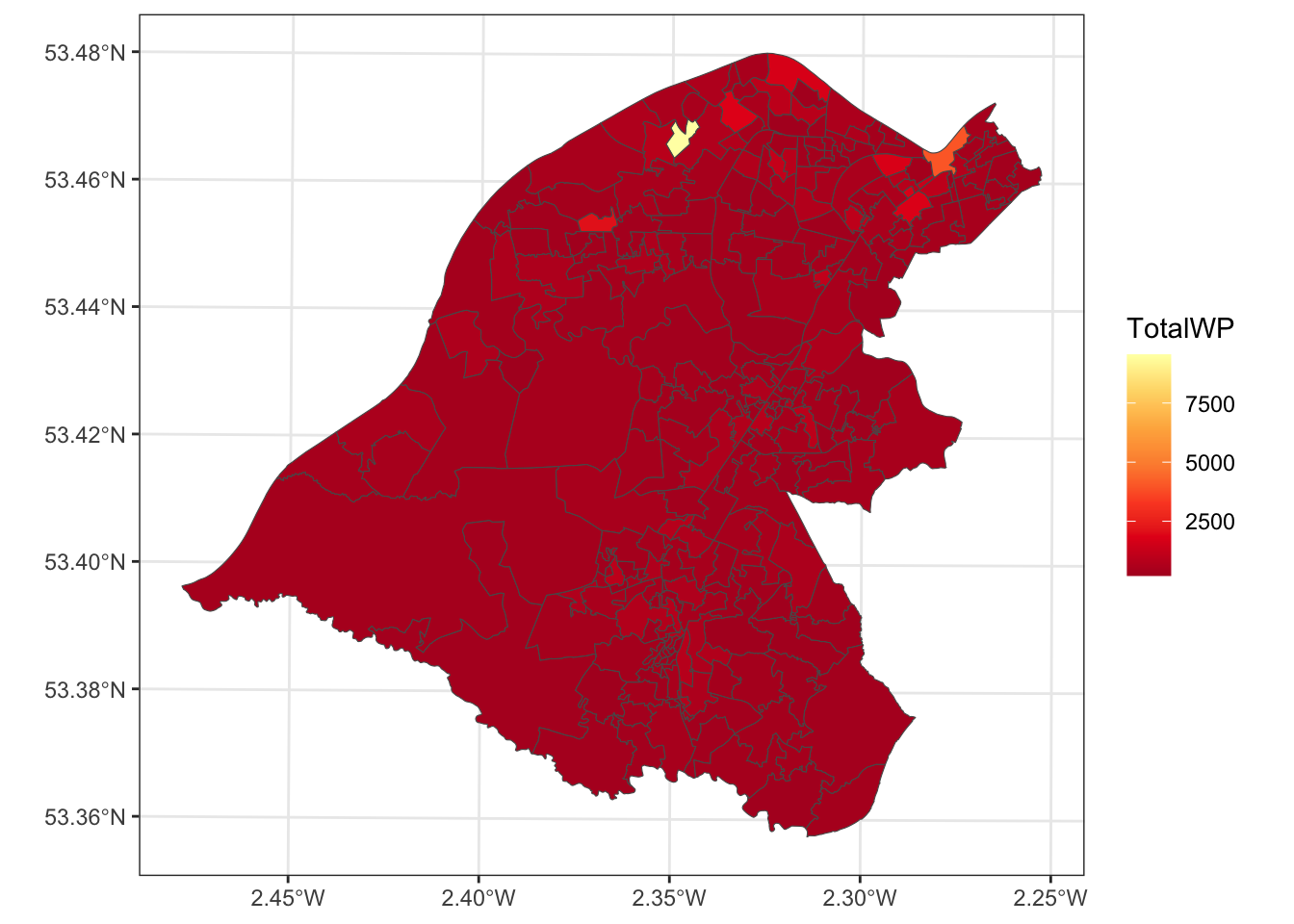
Figure 9.4: Workplace zone populations in Trafford.
head(stores)## StoreID Brand Category Town Suburb Postcode
## 1 0253/0014 ALDI Grocery/Supermarkets MANCHESTER TYLDESLEY M29 8EW
## 2 0253/0001 ALDI Grocery/Supermarkets BIRMINGHAM WARD END B8 2AN
## 3 0253/0008 ALDI Grocery/Supermarkets BIRMINGHAM BORDESLEY GREEN B9 5SP
## 4 0253/0002 ALDI Grocery/Supermarkets SOLIHULL SHIRLEY B90 3AE
## 5 0253/6005 ALDI Grocery/Supermarkets WHITEHAVEN CA28 9DL
## 6 0253/6037 ALDI Grocery/Supermarkets WOLVERHAMPTON WV2 3HP
## Grid_East Grid_North Floorspace..sqft.
## 1 368835.00 402119.00 3040
## 2 412535.00 288186.00 4000
## 3 412125.00 286841.00 4000
## 4 411894.00 279150.00 5000
## 5 297192.00 517643.00 5000
## 6 391642.00 296564.00 59009.4.1 Data preparation
Here we are interested in convenience store locations as we want to find locations for 3 new ones. We need to filter out records / observations that are not in the Trafford area in Manchester. The code below creates a 2km buffer around the workplace zones in Figure 9.4, a spatial layer from the stores data using Easting and Northing (these are in OSGB projection) and the clips the stores spatial layer with the buffer:
# convert to numeric
stores$Grid_East = as.numeric(as.character((stores$Grid_East)))
## Warning: NAs introduced by coercionstores$Grid_North = as.numeric(as.character((stores$Grid_North)))## Warning: NAs introduced by coercion# get rid of NAs
index = !is.na(stores$Grid_North)
# create spatial layer
stores_sf = st_as_sf(stores[index,], coords = c("Grid_East", "Grid_North"), crs = 27700)
# trim down fields
stores_sf$type = "existing"
stores_sf = stores_sf[,9]
# Create 2km spatial data for Trafford areas
wz_buffer = st_buffer(st_union(wz), 2000)
# clip out Trafford stores
stores_sf = stores_sf[wz_buffer,]We can examine these existing locations:
tm_shape(stores_sf) + tm_dots(col = "red", size = 1) +
  tm_shape(wz) + tm_borders()
Next, we need to create some potential locations for the new stores. The st_make_grid functions is very handy for this. The code below defines a hexagonal grid based on the extent of the wz layer, adds a type variable (potential) and joins this to the stores layer defined above, before existing and potential store locations are mapped as in Figure 9.5.
grid = st_make_grid(wz, 500, what = "centers", crs = 27700, square = F)
# make an attribute table for grid
sup_pt = data.frame(type = rep("potential",length(grid)))
# add the grid geometry to it
st_geometry(sup_pt) = grid
# join to existing
supply = rbind(stores_sf,sup_pt)
# clip to 2km buffer
supply = supply[wz_buffer,]
# and plot
p1 = tm_shape(wz) + tm_borders() +
    tm_shape(supply %>% filter(type == "existing") ) + tm_dots(col = "red", size = 0.3) +
    tm_layout(title = "Existing")
# potential sites
p2 = tm_shape(wz) + tm_borders() +
    tm_shape(supply %>% filter(type == "potential") ) + tm_dots(col = "blue", size = 0.05) +
    tm_layout(title = "Potential")
tmap_arrange(p1,p2)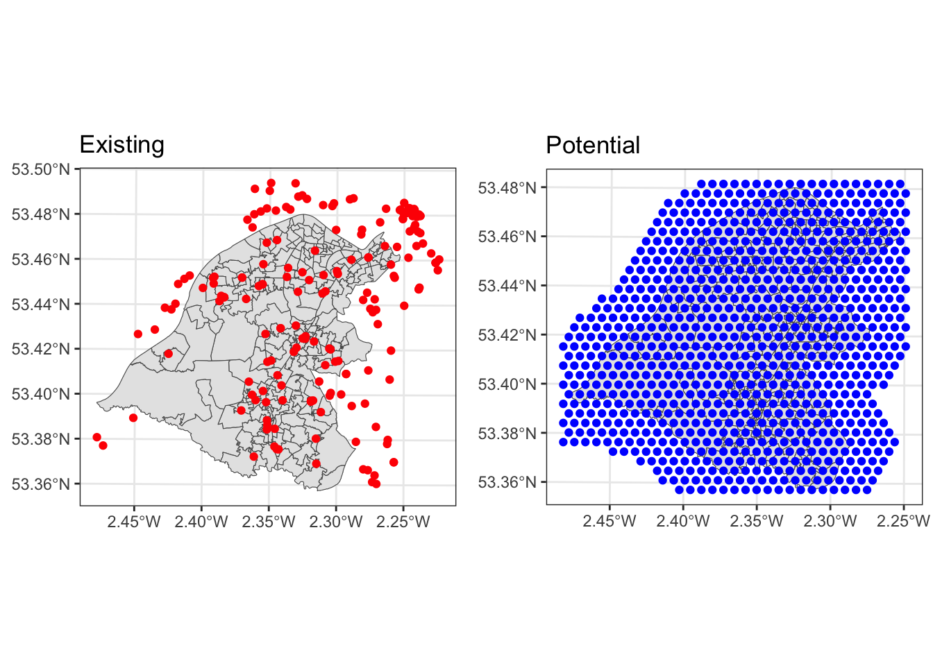
Figure 9.5: The existing and potential supply locations.
9.4.2 Weighted Distance
In order to undertake the location allocation we need a create some kind of distance weighted measure between the supply and demand points. What the allocation will do is try to minimise the sum of this (i.e. the sum of the weighted distance between all supply and the allocated demand). This is important to bare in mind as there may be some situations where you may wish to maximise some objective function. This is needed to evaluate potential supply location (as in the existing and potential supply locations) with respect to demand (as in the workplace zones). The code below create a distance matrix between the workplace zones and the supply locations:
# create distance matrix
d.mat <- (st_distance(wz, supply)/1000)
dim(d.mat)
## [1] 256 1051dim(wz)## [1] 256 5dim(supply)## [1] 1051 2This is a non-symmetrical matrix of the distances (in km) between each Workplace Zone (rows) and each Supply point (columns). Have a look at the first 6 rows and columns:
d.mat[1:6, 1:6]## Units: [m]
## [,1] [,2] [,3] [,4] [,5] [,6]
## [1,] 4.473153 4.210723 1.5730894 6.833619 7.399387 4.625622
## [2,] 3.000913 2.545830 0.9863612 5.145449 8.485449 5.048200
## [3,] 2.431667 2.231559 1.6593746 4.588194 8.512392 4.911704
## [4,] 2.733473 2.968681 1.9862941 5.232414 7.831771 4.339954
## [5,] 3.055995 3.133407 1.8667712 5.488943 7.708793 4.316246
## [6,] 1.770215 2.719927 2.7966096 4.569147 7.903153 4.235837Now the distances need to be weighted by the demand, in this case the TotalWP variable in wz:
# determine the demand weights
w <- wz$TotalWP
# have a look
head(w)
## [1] 9547 1001 886 335 378 200And the distance matrix is multiplied such that it records ‘person distances’. In this case these are in person kilometres but the units are not important. Instead is the relative measures that the location-allocation algorithm uses.
d.mat <- d.mat * wAgain have a look at the first 6 rows and columns and consider how they relate to weight data
d.mat[1:6, 1:6]9.4.3 Undertaking the allocation
We need an index of the existing stores to pass to the allocation function. The idea is that the existing stores are kept in the solution as the algorithm searches to identifies sets of new locations.
keep.index = which(supply$type == "existing")
head(keep.index)
## [1] 1 2 3 4 5 6length(keep.index)## [1] 178There is a small further preparatory step: there are 115 existing stores. If we want to find the locations for 3 new stores
we need to set the parameter p to be \(115+3\) as well as passing the index of the ones we are are keeping (in keep.index).
# define how many to keep
p = length(keep.index) + 3
We can now pass the population / demand weighted distance matrix into the allocate function, noting that the spatial data have to be converted from SF to SP format for this. This may take some time to run.
# allocate
allocations.list2 = allocate(swdf1 = as(wz, "Spatial"),
                 swdf2 = as(supply, "Spatial"),
                 force = keep.index,
                 p=p,
                 metric = d.mat,
                 verbose = F)
# determine the indicates of the new locations
new_store_index = setdiff(allocations.list2, keep.index)
The new store locations can be plotted as well as the areas and supply points:
tm_shape(supply) + tm_dots(col = "white") +
  tm_shape(wz) + tm_polygons(col = "lightyellow") +
    tm_shape(supply[c(allocations.list2, keep.index),]) +
  tm_dots("type", title = "Type of Site", size = 0.3, palette = "Set1") +
  tm_layout(title = "New Supply Sites",
            frame = T, legend.outside = F,
            legend.hist.width = 1,
            legend.format = list(digits = 1),
            legend.position = c("left", "top"),
            legend.text.size = 0.7,
            legend.title.size = 1)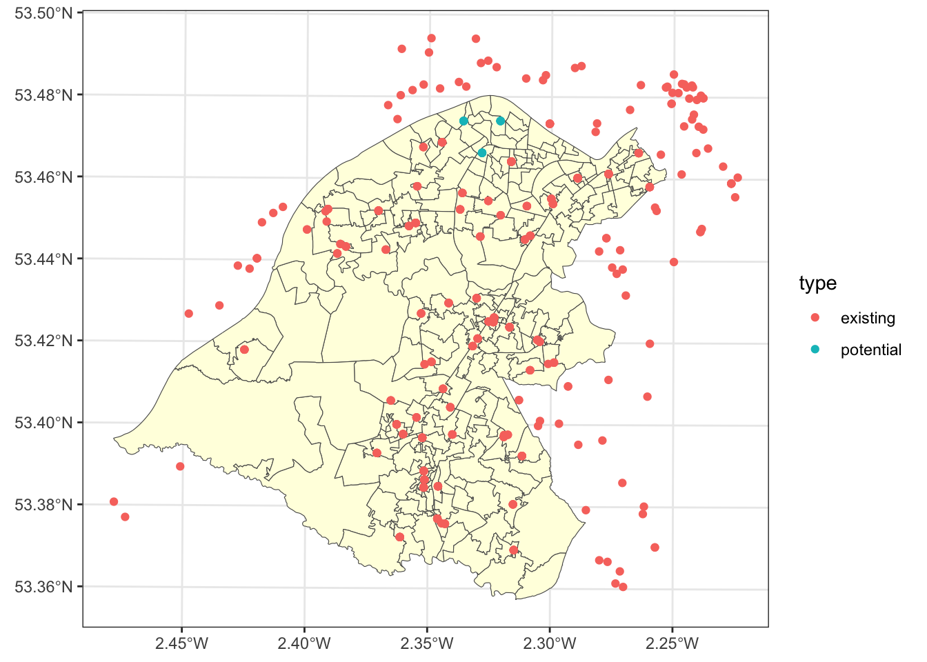
Figure 9.6: The new and existing allocations.
In this case it is possible to plot the allocations as before due, but this time including the supply layer as well as the second argument. However, many of the lines are short, due to the high number of existing supply locations and the low number of allocations - they are not that dramatic!
# create allocations
wz_allocs <- allocations(as(wz, "Spatial"), as(supply, "Spatial"),
                         p=73,force=unique(allocations.list2))
# convert to sf
wz_allocs = st_as_sf(wz_allocs)
# star lines
star_lines <- create_star_lines(wz_allocs, supply)
## Warning in st_centroid.sf(sf1): st_centroid assumes attributes are constant over
## geometries of x## Warning in st_centroid.sf(sf2): st_centroid assumes attributes are constant over
## geometries of xzones = st_union_by(wz, allocations.list2)
p1 = tm_shape(wz) + tm_borders(col = "lightgrey") +
tm_shape(star_lines)+tm_lines(col = "darkred", lwd = 2)
# distance to allocation
p2 = tm_shape(wz_allocs) +
tm_polygons(col = "allocdist",
title = "Distance",
palette = "Reds", n = 7, style = "kmeans")
tmap_arrange(p1, p2)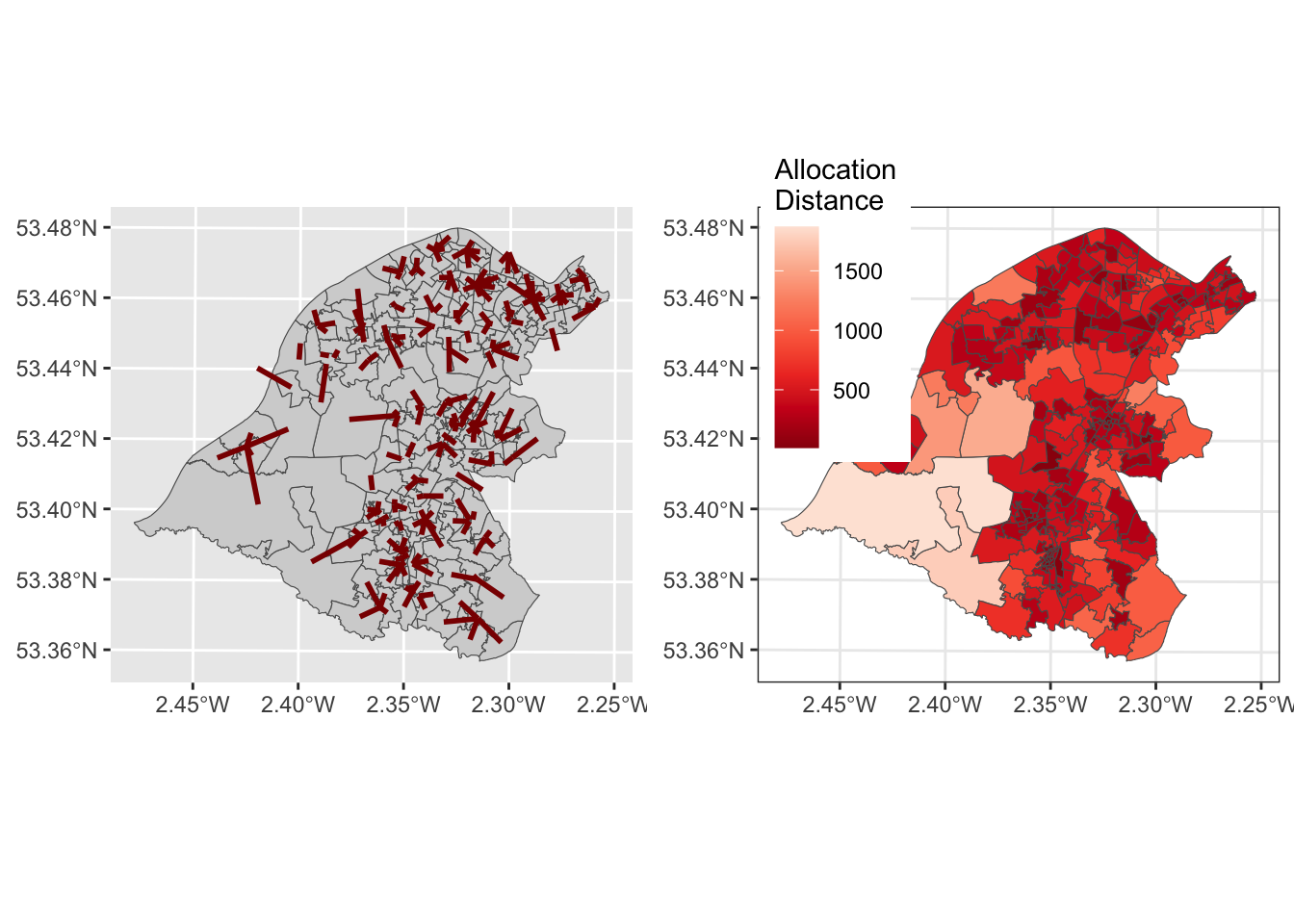
Figure 9.7: The results of the allocations for Trafford, showing the allocation lines and distances.
Finally we can determine the allocation of populations (demand) to the supply. The allocations.list2 object indicates the grouping of the Workplace Zones and they have the customer population
# 1. the original stores
wz$allocation = allocations.list2
wz %>% st_drop_geometry() %>% group_by(allocation) %>%
  summarise(Customers = sum(TotalWP)) %>% data.frame() -> store_customers
summary(store_customers$Customers)
## Min. 1st Qu. Median Mean 3rd Qu. Max.
## 294 702 1130 1780 1885 11224# 2. the new stores
wz$allocation = match(allocations.list2, new_store_index)
wz %>% st_drop_geometry() %>% group_by(allocation) %>%
summarise(Customers = sum(TotalWP)) %>% na.omit() %>% data.frame() -> new_store_customers
new_store_customers## allocation Customers
## 1 1 4340
## 2 2 2948
## 3 3 3726They all look pretty healthy!