Ex. 1

(a) Using “scan”

Use scan() to read every single cell in the baseball-salaries-2016.txt file, need to set sep="\t" to avoid a 2-gram term from being separated into two words.
Use data.frame() to create a data.frame (class) by the input vector.
Then use write.csv() and write.table() to export the file.

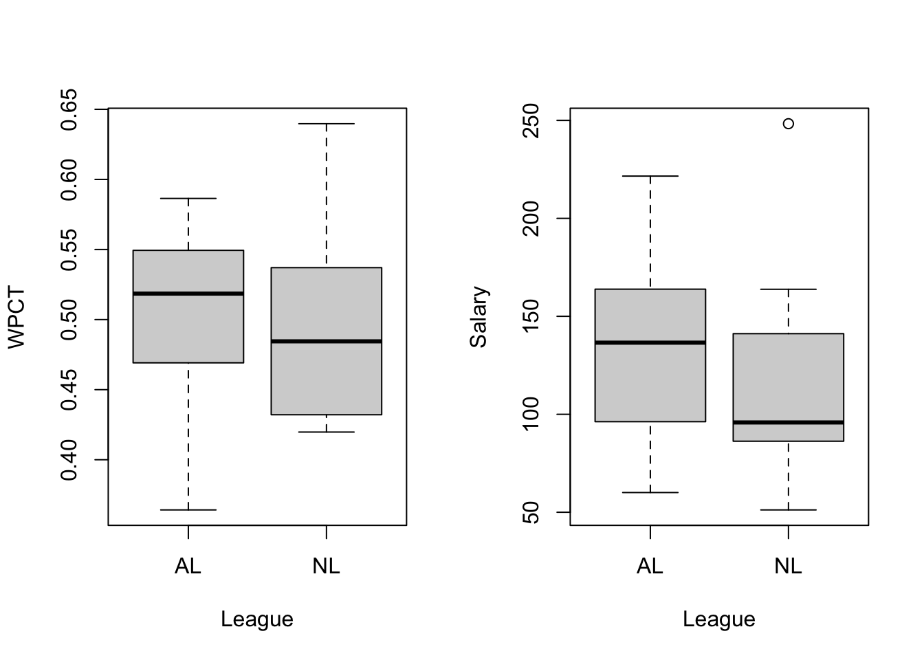
(b) Draw boxplots

salary = Salary ($M)
winning percentage (WPCT) = W/(W+L)

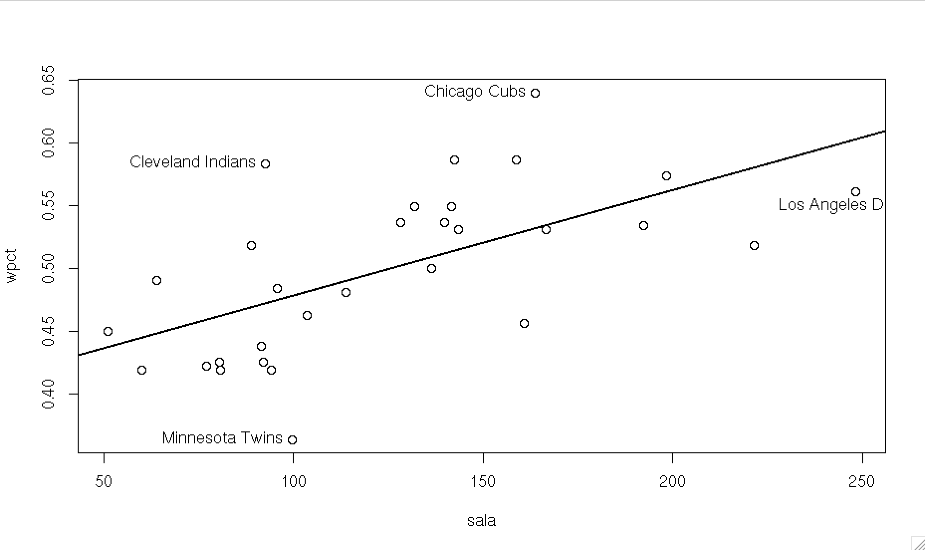
(c) Check correlation

Using cor.test() to check whether the positive relations between salary and winning percentage.
The Pearson’s correlation between salary and winning percentage is 0.617, p<.001, so we can reject the null hypothesis, i.e. the correlation between WPCT and salary is significant.

## 
##  Pearson's product-moment correlation
## 
## data:  sala and wpct
## t = 4.1436, df = 28, p-value = 0.0002856
## alternative hypothesis: true correlation is not equal to 0
## 95 percent confidence interval:
##  0.3294329 0.7992681
## sample estimates:
##       cor 
## 0.6165296

(d) Scatter plot

Ex. 2

(a) Length of a vector

The sample is shown below. When we shorten a vector (set a random seed) from length 20 to 15, only the first 15 numbers would be present. When we lengthen it to 18, three (18-15=3) NAs would be added.

the results of rnorm(20).

##  [1] -1.21  0.28  1.08 -2.35  0.43  0.51 -0.57 -0.55 -0.56 -0.89
## [11] -0.48 -1.00 -0.78  0.06  0.96 -0.11 -0.51 -0.91 -0.84  2.42

the results of length(x) = 15

##  [1] -1.21  0.28  1.08 -2.35  0.43  0.51 -0.57 -0.55 -0.56 -0.89
## [11] -0.48 -1.00 -0.78  0.06  0.96

the results of length(x) = 18

##  [1] -1.21  0.28  1.08 -2.35  0.43  0.51 -0.57 -0.55 -0.56 -0.89
## [11] -0.48 -1.00 -0.78  0.06  0.96    NA    NA    NA

(b) Operations of a vector

Change the $x<0$ part of x[1:20] to NA. The results is shown below.

##  [1]   NA 0.28 1.08   NA 0.43 0.51   NA   NA   NA   NA
## [11]   NA   NA   NA 0.06 0.96   NA   NA   NA   NA 2.42

computing the the mean, median, and variance of non-NA entries in x[1:18] from (a).

## [1] "mean: 0.55"

## [1] "median: 0.47"

## [1] "var: 0.16"

(c) Change NA to 0

using is.na() to identify the NAs, then replaced them by 0s.

##  [1] 0.00 0.28 1.08 0.00 0.43 0.51 0.00 0.00 0.00 0.00
## [11] 0.00 0.00 0.00 0.06 0.96 0.00 0.00 0.00 0.00 2.42

Ex. 3

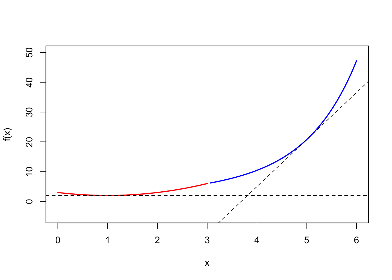
(a) Graph

The graph is shown as 3.(b) below.

(b) Tangent line

Find the slope and intercept of the tangent line of $f(x)=x+2e^{(x-3)}+1$ at $x=5$, then we can use abline() function to draw the tangent line. (Note. in the R abline() function, the intercept is denoted as a, and the slope is denoted as b.)

Slope. $f'(5)=1+2e^{(5-3)}=1+2e^2$
Point. $(x,y)=(5, f(5))=(5, 2e^2+6)$ ( Note. $x=5$ substituted back into the original equation $f(x)$)
Intercept. based on $y=bx+a$, and $b=(1+2e^2)$ is known. (follow the parameters of abline().)

$2e^2+6=5(1+2e^2)+a$, find $a=-8e^2+1$ .

# calculus
expression((x^2-2*x+3), 'x') |> D('x')

## 2 * x - 2

expression((x+2*exp(x-3)+1), 'x') |> D('x')

## 1 + 2 * exp(x - 3)

Ex. 4

(a) `cat()` and `date()`

The codes and outputs are shown below, combine the labels and system time by cat() function.

cat(
  labels = "Today’s date is: ", 
  paste( substr(date(),1,10), substr(date(),21,24)),
  fill = TRUE
)

## Today’s date is:  Tue Mar 22 2022

cat(
  labels = "The time now is: ", 
  paste( substr(date(),12,19)),
  fill = TRUE
)

## The time now is:  23:30:47

(b) Explain the outputs of time.

With the first 2 lines, we assign the system date to the object today (with a class “Date”), then display it as day-month-year format, and the month %b is an abbreviated month in English.
With the 3rd line, we create a sequence that has 10 days, begins today, and generates every other week.
In the 4th line, we extract the weekday name from the object today. In the 5th line, we check every single month’s name from the sequence tenweeks with 10 values.
In the last line, we check the leap seconds (潤秒) before, then display them as the date format.

(today <- Sys.Date())
format(today, "%d %b %Y") 
(tenweeks <- seq(today, length.out=10, by="1 week")) 
weekdays(today) 
months(tenweeks)
as.Date(.leap.seconds)

Ex. 5

(a) Mid-Square Method

By the requirements, the initial values is a 6 digits number, then square it.
How to make sure the 12-digits (square of 6-digits) at the middle of number (including 0, ranging over [0, 999999])? We have introduced the padding method from the stringr package.
The comment of the gen_5a() function. (1) Create a null vector vec. (2) In the for loop, we consider the input or iterate value may not be 6-digits, so we convert it to a character class first, then use str_pad() function to impute 0 at the left side until 12 digits. (3) Use str_sub() to extract the 6 digits from the 4th number to the 9th. (4) Convert the 6-digit number back into the numeric class. (5) Save the numbers in the vector vec with the ith place.
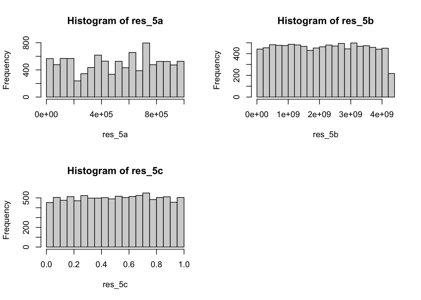
Goodness-of-fit test. We generated 10000 random numbers from the gen_5a() function. The K-S test showed D = 1, p-value < .001, so we reject the null hypothesis, i.e. the random numbers do not follow the uniform distribution.

## Warning in ks.test(res_5a, y = "punif"): ties should not be present for the
## Kolmogorov-Smirnov test

## 
##  One-sample Kolmogorov-Smirnov test
## 
## data:  res_5a
## D = 1, p-value < 2.2e-16
## alternative hypothesis: two-sided

(b) Vax’s generator

The comment of the gen_5b() function. (1) Create a null vector vec. (2) In the for loop, implement a Vax’s generator (69069*x) %% (2^32). (3) Save the numbers in the vector vec with the ith place.
Goodness-of-fit test. We generated 10000 random numbers from the gen_5b() function. For $\chi^2$ test, we separated the 10000 numbers to 10 groups by the intervals of 1/10 of range (max(res_5b) - min(res_5b))/k. Then check the K-S test D = 1, p < .001, we can reject the null hypothesis, i.e. the random numbers do not follow the uniform distribution. However, the $\chi^2$ test showed $\chi^2=6.9936$ with df=9, p=0.6378, we can not reject the null hypothesis, i.e. there are no significant difference between the random numbers and uniform distribution.
K-S test and $\chi^2$ test have different results. But K-S test considers each value, may be better than $\chi^2$ test.

## 
##  One-sample Kolmogorov-Smirnov test
## 
## data:  res_5b
## D = 1, p-value < 2.2e-16
## alternative hypothesis: two-sided

## 
##  Chi-squared test for given probabilities
## 
## data:  chi_5b
## X-squared = 6.9936, df = 9, p-value = 0.6378

(c) Multiplicative congruential generators

The comment of the gen_5c() function. (1) Create a null vector vec. (2) In the for loop, implement a combined generators, (171*x) %% 30269, (172*y) %% 30307, (170*z) %% 30323, and (x/30269 + y/30307 + z/30323) %% 1. (3) Save the numbers in the vector vec with the ith place.
Goodness-of-fit test. We generated 10000 random numbers from the gen_5c() function. Check the K-S test D = 0.010053, p = 0.2643, we can not reject the null hypothesis, i.e. the random numbers do follow the uniform distribution.
Comparison of (a), (b) and (c). We can find the generator of 5(a) and 5(b) can not create a good random numbers iid from uniform distribution (based on K-S test). But the combination generator of 5(c) can do it, because it has a longer cycle.

## 
##  One-sample Kolmogorov-Smirnov test
## 
## data:  res_5c
## D = 0.010053, p-value = 0.2643
## alternative hypothesis: two-sided

The histograms of 5(a), 5(b) and 5(c) is shown below.

Ex. 6

(a) `sample` and `ceiling(runif)`

We test a small value (=100) and a large value (=1000000).

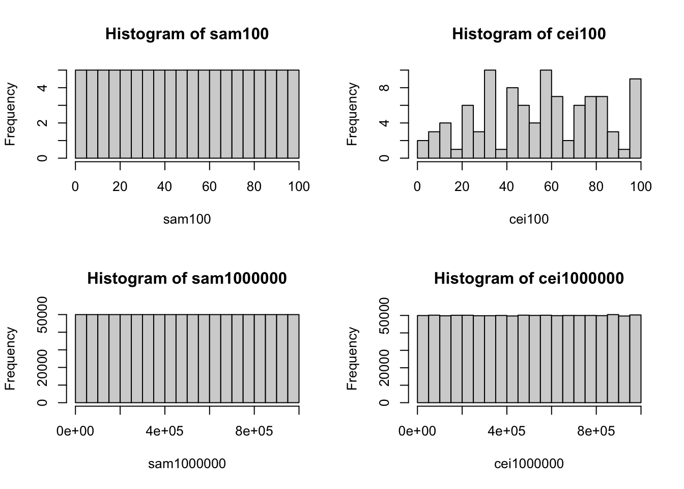
Although these histograms above look very close to uniform distributions. But from the K-S tests, we can find any random numbers created by sample() or ceiling(runif()) are not actually iid from uniform distributions.

## 
##  One-sample Kolmogorov-Smirnov test
## 
## data:  sam100
## D = 1, p-value < 2.2e-16
## alternative hypothesis: two-sided

## Warning in ks.test(x = cei100, y = "punif"): ties should not be present for the
## Kolmogorov-Smirnov test

## 
##  One-sample Kolmogorov-Smirnov test
## 
## data:  cei100
## D = 1, p-value < 2.2e-16
## alternative hypothesis: two-sided

## 
##  One-sample Kolmogorov-Smirnov test
## 
## data:  sam1000000
## D = 1, p-value < 2.2e-16
## alternative hypothesis: two-sided

## Warning in ks.test(x = cei1000000, y = "punif"): ties should not be present for
## the Kolmogorov-Smirnov test

## 
##  One-sample Kolmogorov-Smirnov test
## 
## data:  cei1000000
## D = 1, p-value < 2.2e-16
## alternative hypothesis: two-sided

(b) Hand calculators generator

The comment of the gen_6b() function. (1) Create a null vector vec. (2) In the for loop, implement a generators based on uniform and $\pi$ (pi+u)^5 %% 1. (3) Save the numbers in the vector vec with the ith place.
Goodness-of-fit test. We generated 10000 random numbers from the gen_6b() function. Check the K-S test D = 0.0090575, p = 0.3848, we can not reject the null hypothesis, i.e. the random numbers do follow the uniform distribution.
Compare to #5. In 5(c) we find only the combination generator can create random numbers followed the uniform distribution. Then we check independence by the runs test (from snpar package). The p-value of both res_5c or res_6b is at the 0.05 significance level, so we can conclude that the numbers form them are random (independent).

## 
##  One-sample Kolmogorov-Smirnov test
## 
## data:  res_6b
## D = 0.0090575, p-value = 0.3848
## alternative hypothesis: two-sided

## 
##  Approximate runs rest
## 
## data:  res_5c
## Runs = 5019, p-value = 0.7188
## alternative hypothesis: two.sided

## 
##  Approximate runs rest
## 
## data:  res_6b
## Runs = 4930, p-value = 0.1556
## alternative hypothesis: two.sided

(c) $\phi$ generator

Replaced $pi$ with $\phi=\dfrac{1+\sqrt{5}}{2}$.
Check the K-S test D = 0.0066451, p = 0.7692, we can not reject the null hypothesis, i.e. the random numbers do follow the uniform distribution. And from the runs test with p-value = 0.1676, we can find the numbers are random (independent).

## 
##  One-sample Kolmogorov-Smirnov test
## 
## data:  res_6c
## D = 0.0066451, p-value = 0.7692
## alternative hypothesis: two-sided

## 
##  Approximate runs rest
## 
## data:  res_6c
## Runs = 4932, p-value = 0.1676
## alternative hypothesis: two.sided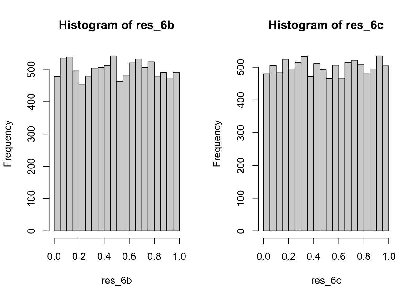

Appendix

Note. After R 4.0, some useful new features are built-in.

The native pipeline syntax |> replaced the tidy-style pipeline %>%.
The shorthand syntax for anonymous functions \(x) is more compact than function(x).

## 1(a) --------
dat1 <- scan('baseball-salaries-2016.txt', what = "character" , sep="\t")
dat1a <- matrix(dat1[-c(1:6)], ncol=6, byrow=T) |> data.frame()
names(dat1a) <- dat1[1:6]

# export data frame
write.csv(dat1a, 'dat1a.csv')
write.table(dat1a, 'dat1a.txt')

## 1(b) --------
dat1b <- rio::import('baseball-salaries-2016.txt')
par(mfrow=c(1,2))
boxplot((W/(W+L)) ~ League, data = dat1b, ylab = 'WPCT' )
boxplot(`Salary ($M)` ~ League, data = dat1b, ylab = 'Salary')

## 1(c) --------
sala <- dat1b$`Salary ($M)`
wpct <- dat1b$W/(dat1b$W+dat1b$L)
team <- dat1b$Team
cor.test(sala, wpct )

## 1(d) --------
x11()
plot(wpct~sala)
abline( lm(wpct~sala) , lwd=2) 
identify(wpct~sala, labels = team)

## 2(a) --------
set.seed(1234)
x_2a = rnorm(20) |> round(2); print(x_2a, width = 65)
length(x_2a) = 15; print(x_2a, width = 65)
length(x_2a) = 18; print(x_2a, width = 65)

## 2(b) --------
set.seed(1234)
x_2a = rnorm(20) |> round(2)
x_2a[x_2a<0] <- NA
print(x_2a, width = 55)

paste0( 'mean: ',mean(x_2a[1:18], na.rm = T) |> round(2) )
paste0( 'median: ', median(x_2a[1:18], na.rm = T) |> round(2) )
paste0( 'var: ', var(x_2a[1:18], na.rm = T) |> round(2) )

## 2(c) --------
x_2a[is.na(x_2a)] <- 0; print(x_2a, width = 55)

## 3(a) 3(b) --------
eq1 <- \(x){ ifelse(x<=3, (x^2-2*x+3), NA) }
eq2 <- \(x){ ifelse(x>3,(x+2*exp(x-3)+1), NA) }

# draw the curves
curve(eq2, from=0, to=6, col='blue', lwd=2,
      ylim = c(-5,50),
      xlab="x", ylab="f(x)")
curve(eq1, from=0, to=6, col='red', lwd=2,
      xlab="x", ylab="f(x)", add = T)

# add some lines
abline( h=2, lty=2 ) 
abline( b=(1+2*exp(2)), a=-8*exp(2)+1, lty=2 )

## 4(a) --------
cat(
  labels = "Today’s date is: ", 
  paste( substr(date(),1,10), substr(date(),21,24)),
  fill = TRUE
)

cat(
  labels = "The time now is: ", 
  paste( substr(date(),12,19)),
  fill = TRUE
)

## 5(a) --------
library('stringr')
  # x= initial value, k=length, vec=random number vector
gen_5a <- \(x, k){
  vec <- c()
  for (i in 1:k){
    x <- as.character(x^2) |>
      stringr::str_pad( width=12, side='left', pad='0' ) |>
      stringr::str_sub(4, 9) |> 
      as.numeric()
    vec[i] <- x
  }
  return(vec)
}

set.seed(1234)
res_5a <- gen_5a( floor( runif(1)*(10^6) ), 10000 )
print( ks.test(res_5a, y="punif") )

## 5(b)--------
gen_5b <- \(x, k){
  vec <- c()
  for(i in 1:k){
    x <- (69069*x) %% (2^32)
    vec[i] <- x
  }
  return(vec)
}

set.seed(1234)
res_5b <- gen_5b( runif(1), k=10000 )

# ks test
print( ks.test(res_5b, y="punif") )

# chisq test

grp_5b <- \(x, k) {
  int <- seq( min(x) , max(x) , (max(res_5b) - min(res_5b))/k )
  vec <- c()
  for (i in 1:k){
    vec[i] <- sum( x<int[i+1] ) - sum( x<int[i] )
  }
  return(vec)
}

chi_5b <- grp_5b( res_5b, k=10 ) 
chisq.test( chi_5b, p= rep(1/10, 10) )

## 5(c) --------
gen_5c <- \(x, y, z){
  vec <- c()
  for(i in 1:10000) {
  x <- (171*x) %% 30269
  y <- (172*y) %% 30307
  z <- (170*z) %% 30323
  u <- (x/30269 + y/30307 + z/30323) %% 1
  vec[i] <- u
}
  return(vec)
} 

res_5c <- gen_5c(x=1, y=2, z=3) 
print( ks.test(res_5c, y="punif") )

# hist
par( mfrow=c(2,2) )
hist(res_5a, 20); hist(res_5b, 20); hist(res_5c, 20)

## 6(a) --------
set.seed(1234)
# 100
sam100 <- sample(100)
cei100 <- ceiling(runif(100)*100)
sam1000000 <- sample(1000000)
cei1000000 <- ceiling(runif(1000000)*1000000)

# graphical 
par(mfrow=c(2,2))
hist(sam100, 20); hist(cei100, 20)
hist(sam1000000, 20); hist(cei1000000, 20)

# test
print(ks.test(x=sam100, y="punif")) 
print(ks.test(x=cei100, y="punif")) 
print(ks.test(x=sam1000000, y="punif")) 
print(ks.test(x=cei1000000, y="punif")) 

## 6(b) --------
set.seed(1234)
gen_6b <- \(k){
  vec <- c()
  u <- runif(1)
  for(i in 1:k){
    u <- (pi+u)^5 %% 1
    vec[i] <- u
  }
  return(vec)
}

res_6b <- gen_6b(10000)
print( ks.test(res_6b, y="punif") )
snpar::runs.test( res_5c )
snpar::runs.test( res_6b )

# 6(c) --------
set.seed(1234)
gen_6c <- \(k){
  vec <- c()
  u <- runif(1)
  phi <- (1+sqrt(5))/2
  for(i in 1:k){
    u <- (phi+u)^5 %% 1
    vec[i] <- u
  }
  return(vec)
}

res_6c <- gen_6c(10000)
print( ks.test(res_6c, y="punif") )
snpar::runs.test( res_6c )

# hist
par(mfrow=c(1,2))
hist(res_6b, 20); hist(res_6c, 20)

[Comp&Simu] Assignment 1

Ex. 1

(a) Using “scan”

(b) Draw boxplots

(c) Check correlation

(d) Scatter plot

Ex. 2

(a) Length of a vector

(b) Operations of a vector

(c) Change NA to 0

Ex. 3

(a) Graph

(b) Tangent line

Ex. 4

(a) `cat()` and `date()`

(b) Explain the outputs of time.

Ex. 5

(a) Mid-Square Method

(b) Vax’s generator

(c) Multiplicative congruential generators

Ex. 6

(a) `sample` and `ceiling(runif)`

(b) Hand calculators generator

(c) \(\phi\) generator

Appendix

[Comp&Simu] Assignment 1

Ex. 1

(a) Using “scan”

(b) Draw boxplots

(c) Check correlation

(d) Scatter plot

Ex. 2

(a) Length of a vector

(b) Operations of a vector

(c) Change NA to 0

Ex. 3

(a) Graph

(b) Tangent line

Ex. 4

(a) cat() and date()

(b) Explain the outputs of time.

Ex. 5

(a) Mid-Square Method

(b) Vax’s generator

(c) Multiplicative congruential generators

Ex. 6

(a) sample and ceiling(runif)

(b) Hand calculators generator

(c) \(\phi\) generator

Appendix

(a) `cat()` and `date()`

(a) `sample` and `ceiling(runif)`