Chapter 2 Introduction to R
This Exploratory Data Analysis section lays the foundation for exploratory data analysis using the R language and packages especially within the tidyverse. This foundation progresses through:
- Introduction : An introduction to the R language
- Abstraction 3 : Exploration of data via reorganization using dplyr 3.4 and other packages in the tidyverse 3.1
- Visualization 4 : Adding visual tools to enhance our data exploration
- Transformation 5 : Reorganizing our data with pivots 5.4 and data joins 5.1

In this chapter we’ll introduce the R language, using RStudio to explore its basic data types, structures, functions and programming methods in base R. We’re assuming you’re either new to R or need a refresher. Later chapters will add packages that extend what you can do with base R for data abstraction, transformation, and visualization, then explore the spatial world, statistical models and time series applied to environmental research.
The following code illustrates a few of the methods we’ll explore in this chapter:
temp <- c(10.7, 9.7, 7.7, 9.2, 7.3)
elev <- c(52, 394, 510, 564, 725)
lat <- c(39.52, 38.91, 37.97, 38.70, 39.09)
elevft <- round(elev / 0.3048)
deg <- as.integer(lat)
min <- as.integer((lat-deg) * 60)
sec <- round((lat-deg-min/60)*3600)
sierradata <- cbind(temp, elev, elevft, lat, deg, min, sec)
mydata <- as.data.frame(sierradata)
mydata
## temp elev elevft lat deg min sec
## 1 10.7 52 171 39.52 39 31 12
## 2 9.7 394 1293 38.91 38 54 36
## 3 7.7 510 1673 37.97 37 58 12
## 4 9.2 564 1850 38.70 38 42 0
## 5 7.3 725 2379 39.09 39 5 24RStudio
If you’re new to RStudio, or would like to learn more about using it, there are plenty of resources you can access to learn more about using it. As with many of the major packages we’ll explore, there’s even a cheat sheet: https://www.rstudio.com/resources/cheatsheets/. Have a look at this cheat sheet while you have RStudio running, and use it to learn about some of its different components:
- The Console where you’ll enter short lines of code, install packages, and get help on functions. Messages created from running code will also be displayed here. There are other tabs in this area (e.g. Terminal, R Markdown) we may explore a bit, but mostly we’ll use the console.
- The Source Editor where you’ll write full R scripts and R Markdown documents. You should get used to writing complete scripts and R Markdown documents as we go through the book.
- Various Tab Panes such as the Environment pane where you can explore what scalars and more complex objects contain.
- The Plots pane in the lower right for static plots (graphs & maps that aren’t interactive), which also lets you see a listing of Files, or View interactive maps and maps.
2.1 Data Objects
As with all programming 2.8 languages, R works with data and since it’s an object-oriented language, these are data objects. Data objects can range from the most basic type – the scalar which holds one value, like a number or text – to everything from an array of values to spatial data for mapping or a time series of data.
2.1.1 Scalars and Assignment
We’ll be looking at a variety of types of data objects, but scalars are the most basic type, holding individual values, so we’ll start with it. Every computer language, like in math, stores values by assigning them constants or results of expressions. These are often called “variables” but we’ll be using that name to refer to a column of data stored in a data frame, which we’ll look at later in this chapter. R uses a lot of objects, and not all are data objects; we’ll also create functions 2.8.1, a type of object that does something (runs the function code you’ve defined for it) with what you provide it.
To create a scalar (or other data object), we’ll use the most common type of statement, the assignment statement, that takes an expression and assigns it to a new data object that we’ll name. The class of that data object is determined by the class of the expression provided, and that expression might be something as simple as a constant like a number or a character string of text. Here’s an example of a very basic assignment statement that assigns the value of a constant 5 to a new scalar x:
x <- 5
Note that this uses the assignment operator <- that is standard for R. You can also use = as most languages do (and I sometimes do), but we’ll use = for other types of assignments.
All object names must start with a letter, have no spaces, and not use any names that are built into the R language or used in package libraries, such as reserved words like for or function names like log. Object names are case-sensitive (which you’ll probably discover at some point by typing in something wrong and getting an error).
x <- 5
y <- 8
Longitude <- -122.4
Latitude <- 37.8
my_name <- "Inigo Montoya"
To check the value of a data object, you can just enter the name in the console, or even in a script or code chunk.
x## [1] 5y## [1] 8Longitude## [1] -122.4Latitude## [1] 37.8my_name## [1] "Inigo Montoya"This is counter to the way printing out values commonly works in other programming languages, and you will need to know how this method works as well because you will want to use your code to develop tools that accomplish things, and there are also limitations to what you can see by just naming objects.
To see the values of objects in programming mode, you can also use the print() function (but we rarely do); or to concatenate character string output, use paste() or paste0.
print(x)
paste0("My name is ", my_name, ". You killed my father. Prepare to die.")
Numbers concatenated with character strings are converted to characters.
paste0(paste("The Ultimate Answer to Life", "The Universe",
"and Everything is ... ", sep=", "),42,"!")paste("The location is latitude", Latitude, "longitude", Longitude)## [1] "The location is latitude 37.8 longitude -122.4"Review the code above and what it produces. Without looking it up, what’s the difference between paste() and paste0()?
We’ll use
paste0()a lot in this book to deal with long file path which create problems for the printed/pdf version of this book, basically extending into the margins. Breaking the path into multiple strings and then combining them withpaste0()is one way to handle them. For instance, in the Imagery and Classification Models chapter, the Sentinel2 imagery is provided in a very long file path. So here’s how we usepaste0()to recombine after breaking up the path, and we then take it one more step and build out the full path to the 20 m imagery subset.
imgFolder <- paste0("S2A_MSIL2A_20210628T184921_N0300_R113_T10TGK_20210628T230915.",
                    "SAFE/GRANULE/L2A_T10TGK_A031427_20210628T185628")
img20mFolder <- paste0("~/sentinel2/",imgFolder,"/IMG_DATA/R20m")
2.2 Functions
Just as in regular mathematics, R makes a lot of use of functions that accept an input and create an output:
log10(100)
log(exp(5))
cos(pi)
sin(90 * pi/180)
But functions can be much more than numerical ones, and R functions can return a lot of different data objects. You’ll find that most of your work will involve functions, from those in base R to a wide variety in packages you’ll be adding. You will likely have already used the install.packages() and library() functions that add in an array of other functions.
Later in this chapter, we’ll also learn how to write our own functions, a capability that is easy to accomplish and also gives you a sense of what developing your own package might be like.
Arithmetic operators There are of course all the normal arithmetic operators (that are actually functions) like plus + and minus - or the key-stroke approximations of multiply * and divide / operators. You’re probably familiar with these approximations from using equations in Excel if not in some other programming language you may have learned. These operators look a bit different from how they’d look when creating a nicely formatted equation.
For example, \(\frac{NIR - R}{NIR + R}\) instead has to look like (NIR-R)/(NIR+R).
Similarly * must be used to multiply; there’s no implied multiplication that we expect in a math equation like \(x(2+y)\) which would need to be written x*(2+y).
In contrast to those four well-known operators, the symbol used to exponentiate – raise to a power – varies among programming languages. R uses either ** or ^ so the the Pythagorean theorem \(c^2=a^2+b^2\) might be written c**2 = a**2 + b**2 or c^2 = a^2 + b^2 except for the fact that it wouldn’t make sense as a statement to R. Why?
And how would you write an R statement that assigns the variable c an expression derived from the Pythagorean theorem? (And don’t use any new functions from a Google search – from deep math memory, how do you do \(\sqrt{x}\) using an exponent?)
It’s time to talk more about expressions and statements.
2.3 Expressions and Statements
The concepts of expressions and statements are very important to understand in any programming language.
An expression in R (or any programming language) has a value just like an object has a value. An expression will commonly combine data objects and functions to be evaluated to derive the value of the expression. Here are some examples of expressions:
5
x
x*2
sin(x)
(a^2 + b^2)^0.5
(-b+sqrt(b**2-4*a*c))/2*a
paste("My name is", aname)
Note that some of those expressions used previously assigned objects – x, a, b, c, aname.
An expression can be entered in the console to display its current value, and this is commonly done in R for objects of many types and complexity.
cos(pi)## [1] -1Nile## Time Series:
## Start = 1871
## End = 1970
## Frequency = 1
## [1] 1120 1160 963 1210 1160 1160 813 1230 1370 1140 995 935 1110 994 1020
## [16] 960 1180 799 958 1140 1100 1210 1150 1250 1260 1220 1030 1100 774 840
## [31] 874 694 940 833 701 916 692 1020 1050 969 831 726 456 824 702
## [46] 1120 1100 832 764 821 768 845 864 862 698 845 744 796 1040 759
## [61] 781 865 845 944 984 897 822 1010 771 676 649 846 812 742 801
## [76] 1040 860 874 848 890 744 749 838 1050 918 986 797 923 975 815
## [91] 1020 906 901 1170 912 746 919 718 714 740Whoa, what was that? We entered the expression Nile and got a bunch of stuff! Nile is a type of data object called a time series that we’ll be looking at much later, and since it’s in the built-in data in base R, just entering its name will display it. And since time series are also vectors which are like entire columns, rows or variables of data, we can vectorize it (apply mathematical operations and functions element-wise) in an expression:
Nile * 2## Time Series:
## Start = 1871
## End = 1970
## Frequency = 1
## [1] 2240 2320 1926 2420 2320 2320 1626 2460 2740 2280 1990 1870 2220 1988 2040
## [16] 1920 2360 1598 1916 2280 2200 2420 2300 2500 2520 2440 2060 2200 1548 1680
## [31] 1748 1388 1880 1666 1402 1832 1384 2040 2100 1938 1662 1452 912 1648 1404
## [46] 2240 2200 1664 1528 1642 1536 1690 1728 1724 1396 1690 1488 1592 2080 1518
## [61] 1562 1730 1690 1888 1968 1794 1644 2020 1542 1352 1298 1692 1624 1484 1602
## [76] 2080 1720 1748 1696 1780 1488 1498 1676 2100 1836 1972 1594 1846 1950 1630
## [91] 2040 1812 1802 2340 1824 1492 1838 1436 1428 1480More on that later, but we’ll start using vectors here and there. Back to expressions and statements:
A statement in R does something. It represents a directive we’re assigning to the computer, or maybe the environment we’re running on the computer (like RStudio, which then runs R). A simple print() statement seems a lot like what we just did when we entered an expression in the console, but recognize that it does something:
print("Hello, World")## [1] "Hello, World"Which is the same as just typing "Hello, World", but either way we write it, it does something.
Statements in R are usually put on one line, but you can use a semicolon to have multiple statements on one line, if desired:
x <- 5; print(x); print(x**2); x; x^0.5## [1] 5## [1] 25## [1] 5## [1] 2.236068What’s the print function for? It appears that you don’t really need a print function, since you can just enter an object you want to print in a statement, so the print() is implied. And indeed we’ll rarely use it, though there are some situations where it’ll be needed, for instance in a structure like a loop. It also has a couple of parameters you can use like setting the number of significant digits:
print(x^0.5, digits=3)## [1] 2.24Many (perhaps most) statements don’t actually display anything. For instance:
x <- 5doesn’t display anything, but it does assign the constant 5 to the object x, so it simply does something. It’s an assignment statement, easily the most common type of statement that we’ll use in R, and uses that special assignment operator <- . Most languages just use = which the designers of R didn’t want to use, to avoid confusing it with the equal sign meaning “is equal to”.
An assignment statement assigns an expression to a object. If that object already exists, it is reused with the new value. For instance it’s completely legit (and commonly done in coding) to update the object in an assignment statement. This is very common when using a counter scalar:
i = i + 1You’re simply updating the index object with the next value. This also illustrates why it’s not an equation: i=i+1 doesn’t work as an equation (unless i is actually \(\infty\) but that’s just really weird.)
And c**2 = a**2 + b**2 doesn’t make sense as an R statement because c**2 isn’t an object to be created. The ** part is interpreted as raise to a power. What is to the left of the assignment operator = must be an object to be assigned the value of the expression.
2.4 Data Classes
Scalars, constants, vectors and other data objects in R have data classes. Common types are numeric and character, but we’ll also see some special types like Date.
x <- 5
class(x)
## [1] "numeric"class(4.5)## [1] "numeric"class("Fred")## [1] "character"class(as.Date("2021-11-08"))## [1] "Date"2.4.1 Integers
By default, R creates double-precision floating-point numeric data objects To create integer objects:
- append an L to a constant, e.g.
5Lis an integer 5 - convert with
as.integer
We’re going to be looking at various as. functions in R, more on that later, but we should look at as.integer() now. Most other languages use int() for this, and what it does is converts any number into an integer, truncating it to an integer, not rounding it.
as.integer(5)## [1] 5as.integer(4.5)## [1] 4To round a number, there’s a round() function or you can instead use as.integer adding 0.5:
x <- 4.8
y <- 4.2
as.integer(x + 0.5)
## [1] 5round(x)## [1] 5as.integer(y + 0.5)## [1] 4round(y)## [1] 4Integer division is really the first kind of division you learned about in elementary school, and is the kind of division that each step in long division employs, where you first get the highest integer you can get …
5 %/% 2## [1] 2… but then there’s a remainder from division, which we can call the modulus. To see the modulus we use %% instead of %/%:
5 %% 2## [1] 1That modulus is handy for periodic data (like angles of a circle, hours of the day, days of the year), where if we use the length of that period (like 360°) as the divisor, the remainder will always be the value’s position in the repeated period. We’ll use a vector created by the seq function, and then apply a modulus operation:
ang = seq(90,540,90)
ang
## [1] 90 180 270 360 450 540ang %% 360## [1] 90 180 270 0 90 180Surprisingly, the values returned by integer division or the remainder are not stored as integers. R seems to prefer floating point…
2.5 Rectangular data
A common data format used in most types of research is rectangular data such as in a spreadsheet, with rows and columns, where rows might be observations and columns might be variables (Figure 2.1). We’ll read this type of data in from spreadsheets or even more commonly from comma-separated-variable (CSV) files, though some of these package data sets are already available directly as data frames.
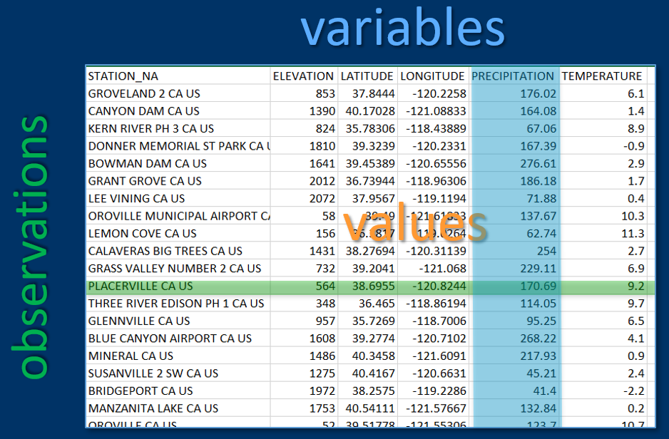
FIGURE 2.1: Variables, observations and values in rectangular data
library(igisci)
sierraFeb
## # A tibble: 82 × 7
## STATION_NAME COUNTY ELEVA…¹ LATIT…² LONGI…³ PRECI…⁴ TEMPE…⁵
## <chr> <chr> <dbl> <dbl> <dbl> <dbl> <dbl>
## 1 GROVELAND 2, CA US Tuolu… 853. 37.8 -120. 176. 6.1
## 2 CANYON DAM, CA US Plumas 1390. 40.2 -121. 164. 1.4
## 3 KERN RIVER PH 3, CA US Kern 824. 35.8 -118. 67.1 8.9
## 4 DONNER MEMORIAL ST PARK, CA US Nevada 1810. 39.3 -120. 167. -0.9
## 5 BOWMAN DAM, CA US Nevada 1641. 39.5 -121. 277. 2.9
## 6 BRUSH CREEK RANGER STATION, C… Butte 1085. 39.7 -121. 296. NA
## 7 GRANT GROVE, CA US Tulare 2012. 36.7 -119. 186. 1.7
## 8 LEE VINING, CA US Mono 2072. 38.0 -119. 71.9 0.4
## 9 OROVILLE MUNICIPAL AIRPORT, C… Butte 57.9 39.5 -122. 138. 10.3
## 10 LEMON COVE, CA US Tulare 156. 36.4 -119. 62.7 11.3
## # … with 72 more rows, and abbreviated variable names ¹ELEVATION, ²LATITUDE,
## # ³LONGITUDE, ⁴PRECIPITATION, ⁵TEMPERATURE2.6 Data Structures in R
We’ve already started using the most common data structures – scalars and vectors – but haven’t really talked about vectors yet, so we’ll start there.
2.6.1 Vectors
A vector is an ordered collection of numbers, strings, vectors, data frames, etc. What we mostly refer to simply as vectors are formally called atomic vectors which requires that they be homogeneous sets of whatever type we’re referring to, such as a vector of numbers,or a vector of strings, or a vector of dates/times.
You can create a simple vector with the c() function:
lats <- c(37.5,47.4,29.4,33.4)
lats
## [1] 37.5 47.4 29.4 33.4states <- c("VA", "WA", "TX", "AZ")
states## [1] "VA" "WA" "TX" "AZ"zips <- c(23173, 98801, 78006, 85001)
zips## [1] 23173 98801 78006 85001The class of a vector is the type of data it holds
temp <- c(10.7, 9.7, 7.7, 9.2, 7.3, 6.7)
class(temp)
## [1] "numeric"Let’s also introduce the handy str() function which in one step gives you a view of the class of an item and its content, so its structure. We’ll often use it in this book when we want to tell the reader what a data object contains, instead of listing a vector and its class separately, so instead of …
temp## [1] 10.7 9.7 7.7 9.2 7.3 6.7class(temp)## [1] "numeric"… we’ll just use str():
str(temp)## num [1:6] 10.7 9.7 7.7 9.2 7.3 6.7Vectors can only have one data class, and if mixed with character types, numeric elements will become character:
mixed <- c(1, "fred", 7)
str(mixed)
## chr [1:3] "1" "fred" "7"mixed[3] # gets a subset, example of coercion## [1] "7"2.6.1.1 NA
Data science requires dealing with missing data by storing some sort of null value, called various things:
- null
- nodata
NA“not available” or “not applicable”
as.numeric(c("1","Fred","5")) # note NA introduced by coercion## [1] 1 NA 5We often want to ignore NA in statistical summaries. Where normally the summary statistic can only return NA…
mean(as.numeric(c("1", "Fred", "5")))## [1] NA… with na.rm=T you can still get the result for all actual data:
mean(as.numeric(c("1", "Fred", "5")), na.rm=T)## [1] 3Don’t confuse with nan (“not a number”) which is used for things like imaginary numbers (explore the help for more on this)
is.nan(NA)## [1] FALSEis.na(as.numeric(''))## [1] TRUEis.nan(as.numeric(''))## [1] FALSEi <- sqrt(-1)
is.na(i) # interestingly nan is also na## [1] TRUEis.nan(i)## [1] TRUE2.6.1.2 Creating a vector from a sequence
We often need sequences of values, and there are a few ways of creating them. The following 3 examples are equivalent:
seq(1,10)
1:10
c(1,2,3,4,5,6,7,8,9,10)
The seq() function has special uses like using a step parameter:
seq(2,10,2)## [1] 2 4 6 8 102.6.1.3 Vectorization and vector arithmetic
Arithmetic on vectors operates element-wise, a process called vectorization.
elev <- c(52,394,510,564,725,848,1042,1225,1486,1775,1899,2551)
elevft <- elev / 0.3048
elevft
## [1] 170.6037 1292.6509 1673.2283 1850.3937 2378.6089 2782.1522 3418.6352
## [8] 4019.0289 4875.3281 5823.4908 6230.3150 8369.4226Another example, with 2 vectors:
temp03 <- c(13.1,11.4,9.4,10.9,8.9,8.4,6.7,7.6,2.8,1.6,1.2,-2.1)
temp02 <- c(10.7,9.7,7.7,9.2,7.3,6.7,4.0,5.0,0.9,-1.1,-0.8,-4.4)
tempdiff <- temp03 - temp02
tempdiff
## [1] 2.4 1.7 1.7 1.7 1.6 1.7 2.7 2.6 1.9 2.7 2.0 2.32.6.1.4 Plotting vectors
Vectors of Feb temperature, elevation and latitude at stations in the Sierra:
temp <- c(10.7,  9.7,  7.7,  9.2,  7.3,  6.7,  4.0,  5.0,  0.9, -1.1, -0.8,-4.4)
elev <-   c(52,  394,  510,  564,  725,  848, 1042, 1225, 1486, 1775, 1899, 2551)
lat <- c(39.52,38.91,37.97,38.70,39.09,39.25,39.94,37.75,40.35,39.33,39.17,38.21)
Plot individually by index vs a scatterplot
We’ll use the plot() function to visualize what’s in a vector. The plot() function will create an output based upon its best guess of what you’re wanting to see, and will depend on the nature of the data you provide it. We’ll be looking at a lot of ways to visualize data soon, but it’s often useful to just see what plot() gives you. In this case it just makes a bivariate plot where the x dimension is the sequential index of the vector from 1 through the length of the vector, and the values are in the y dimension. For comparison is a scatterplot with elevation on the x axis (Figure 2.2).
plot(temp)
plot(elev,temp)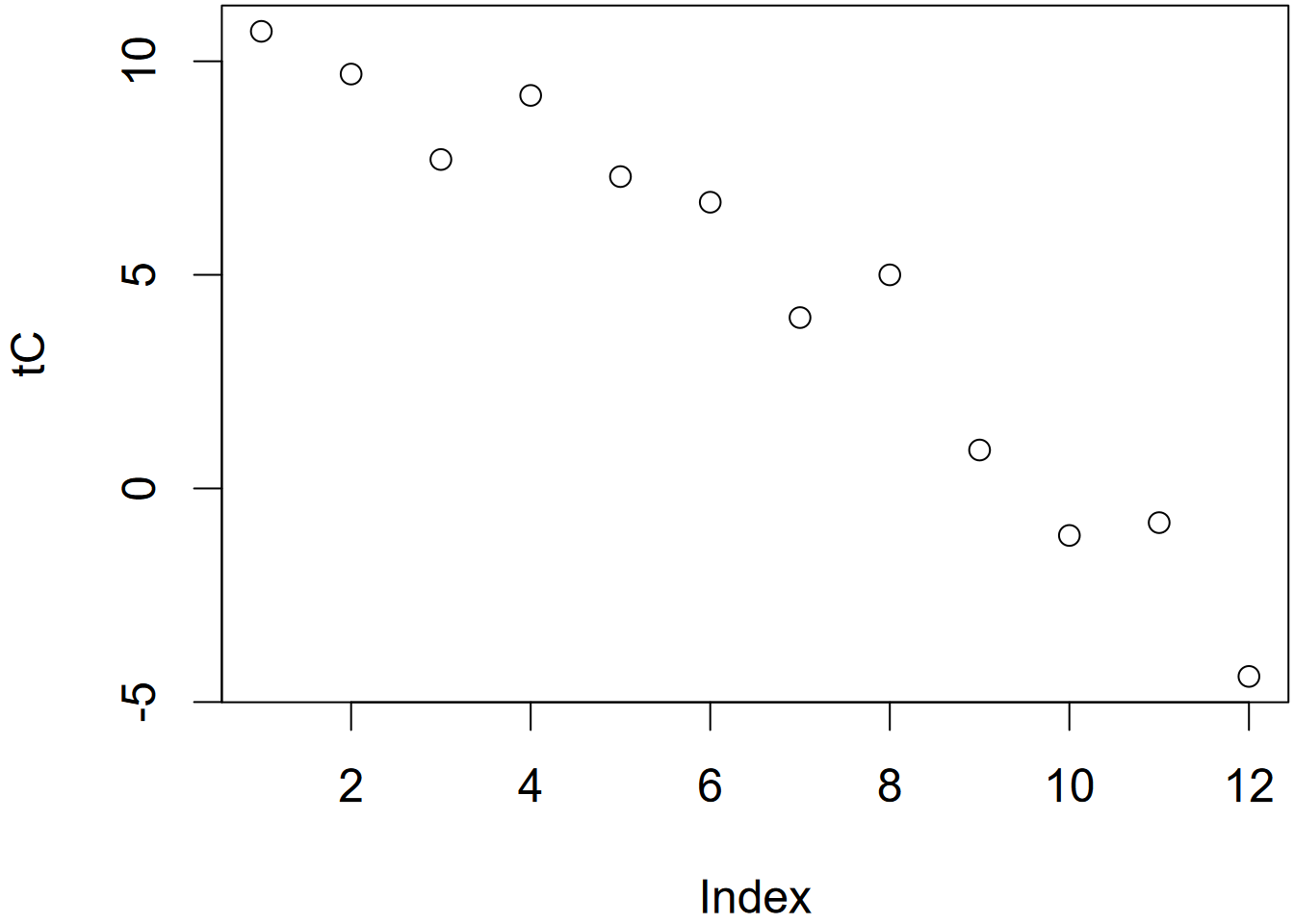
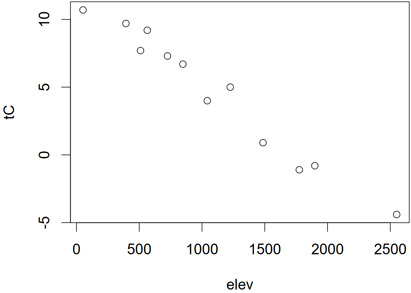
FIGURE 2.2: Temperature plotted by index (left) and elevation (right)
2.6.1.5 Named indices
Vectors themselves have names (like elev, temp, and lat above), but individual indices can also be named.
fips <- c(16, 30, 56)
str(fips)
## num [1:3] 16 30 56fips <- c(idaho = 16, montana = 30, wyoming = 56)
str(fips)## Named num [1:3] 16 30 56
## - attr(*, "names")= chr [1:3] "idaho" "montana" "wyoming"The reason we might do this is so you can refer to observations by name instead of index, maybe to filter observations based on criteria where the name will be useful. The following are equivalent:
fips[2]## montana
## 30fips["montana"]## montana
## 30The names() function can be used to display a character vector of names, or assign names from a character vector:
names(fips) # returns a character vector of names## [1] "idaho" "montana" "wyoming"names(fips) <- c("Idaho","Montana","Wyoming")
names(fips)## [1] "Idaho" "Montana" "Wyoming"2.6.2 Lists
Lists can be heterogeneous, with multiple class types. Lists are actually used a lot in R, and are created by many operations, but they can be confusing to get used to especially when it’s unclear what we’ll be using them for. We’ll avoid them for a while, and look into specific examples as we need them.
2.6.3 Matrices
Vectors are commonly used as a column in a matrix (or as we’ll see, a data frame), like a variable
temp <- c(10.7,  9.7,  7.7,  9.2,  7.3,  6.7,  4.0,  5.0,  0.9, -1.1, -0.8,-4.4)
elev <-   c(52,  394,  510,  564,  725,  848, 1042, 1225, 1486, 1775, 1899, 2551)
lat <- c(39.52,38.91,37.97,38.70,39.09,39.25,39.94,37.75,40.35,39.33,39.17,38.21)
Building a matrix from vectors as columns
sierradata <- cbind(temp, elev, lat)
class(sierradata)
## [1] "matrix" "array"str(sierradata)## num [1:12, 1:3] 10.7 9.7 7.7 9.2 7.3 6.7 4 5 0.9 -1.1 ...
## - attr(*, "dimnames")=List of 2
## ..$ : NULL
## ..$ : chr [1:3] "temp" "elev" "lat"sierradata## temp elev lat
## [1,] 10.7 52 39.52
## [2,] 9.7 394 38.91
## [3,] 7.7 510 37.97
## [4,] 9.2 564 38.70
## [5,] 7.3 725 39.09
## [6,] 6.7 848 39.25
## [7,] 4.0 1042 39.94
## [8,] 5.0 1225 37.75
## [9,] 0.9 1486 40.35
## [10,] -1.1 1775 39.33
## [11,] -0.8 1899 39.17
## [12,] -4.4 2551 38.212.6.3.1 Dimensions for arrays and matrices
Note: a matrix is just a 2D array. Arrays have 1, 3, or more dimensions.
dim(sierradata)## [1] 12 3It’s also important to remember that a matrix or an array is a vector with dimensions, and we can change those dimensions in various ways as long as they work for the length of the vector.
a <- 1:12
dim(a) <- c(3, 4)   # matrix
class(a)
## [1] "matrix" "array"dim(a) <- c(2,3,2) # 3D array
class(a)## [1] "array"dim(a) <- 12 # 1D array
class(a)## [1] "array"b <- matrix(1:12, ncol=1) # 1 column matrix is allowedWe just saw that we can change the dimensions of an existing matrix or array. But what if the matrix has names for its columns? I wasn’t sure so following my basic philosophy of empirical programming I just tried it:
dim(sierradata) <- c(3,12)
sierradata
## [,1] [,2] [,3] [,4] [,5] [,6] [,7] [,8] [,9] [,10] [,11] [,12]
## [1,] 10.7 9.2 4.0 -1.1 52 564 1042 1775 39.52 38.70 39.94 39.33
## [2,] 9.7 7.3 5.0 -0.8 394 725 1225 1899 38.91 39.09 37.75 39.17
## [3,] 7.7 6.7 0.9 -4.4 510 848 1486 2551 37.97 39.25 40.35 38.21So the answer is that it gets rid of the column names, and we can also see that redimensioning changes a lot more about how the data appears (though dim(sierradata) <- c(12,3) will return it to its original structure, but without column names). It’s actually a little odd that matrices can have column names, because that really just makes them seem like data frames, so let’s look at those next. Let’s consider a situation where we want to create a rectangular data set from some data for a set of states:
abb <- c("CO","WY","UT")
area <- c(269837, 253600, 84899)
pop <- c(5758736, 578759, 3205958)
We can use cbind to create a matrix out of them, just like we did with the sierradata above
cbind(abb,area,pop)## abb area pop
## [1,] "CO" "269837" "5758736"
## [2,] "WY" "253600" "578759"
## [3,] "UT" "84899" "3205958"But notice what it did – area and pop were converted to character type. This reminds us that matrices are still atomic vectors – all of the same class. So to comply with this, the numbers were converted to character strings, since you can’t convert character strings to numbers.
This isn’t very satisfactory as a data object, so we’ll need to use a data frame, which is not a vector, though its individual column variables are vectors.
2.6.4 Data frames
A data frame is a database with variables in columns and rows of observations. They’re kind of like a spreadsheet with rules (like the first row is field names) or a matrix that can have variables of unique types. Data frames will be very important for data analysis and GIS.
Before we get started, we’re going to use the palmerpenguins data set (Figure 2.3), so you’ll need to install it if you haven’t yet, and I’d encourage you to learn more about it at https://allisonhorst.github.io/palmerpenguins/articles/intro.html(Horst, Hill, and Gorman (2020)). It will be useful for a variety of demonstrations using numerical morphometric variables (Figure 2.4) as well as a couple of categorical factors (species and island).
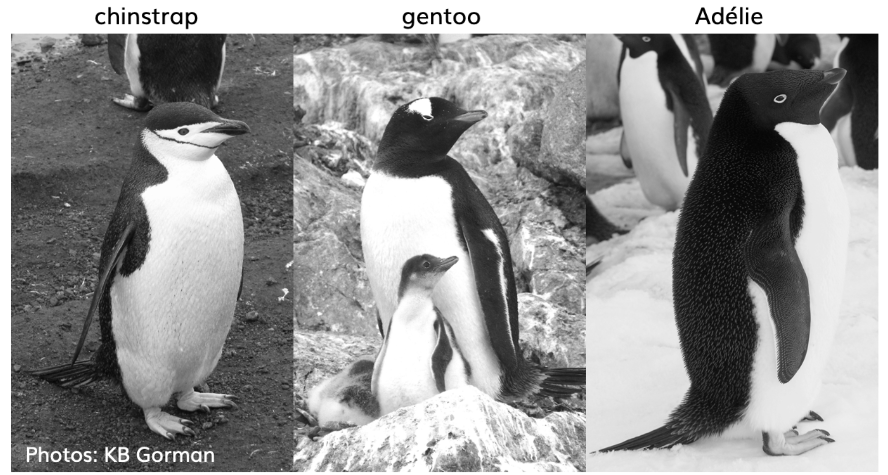
FIGURE 2.3: The three penguin species in palmerpenguins. Photos by KB Gorman. Used with permission
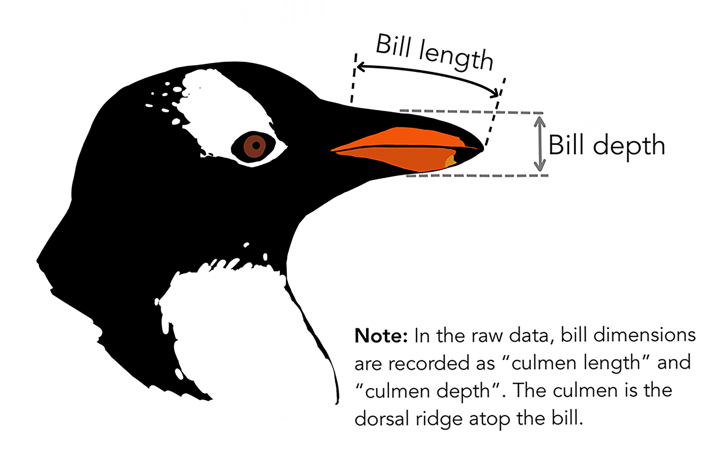
FIGURE 2.4: Diagram of penguin head with indication of bill length and bill depth (from Horst, Hill, and Gorman (2020), used with permission)
We’ll use a couple of alternative table display methods, first a simple one…
library(palmerpenguins)
penguins
## # A tibble: 344 × 8
## species island bill_length_mm bill_depth_mm flipper_…¹ body_…² sex year
## <fct> <fct> <dbl> <dbl> <int> <int> <fct> <int>
## 1 Adelie Torgersen 39.1 18.7 181 3750 male 2007
## 2 Adelie Torgersen 39.5 17.4 186 3800 fema… 2007
## 3 Adelie Torgersen 40.3 18 195 3250 fema… 2007
## 4 Adelie Torgersen NA NA NA NA <NA> 2007
## 5 Adelie Torgersen 36.7 19.3 193 3450 fema… 2007
## 6 Adelie Torgersen 39.3 20.6 190 3650 male 2007
## 7 Adelie Torgersen 38.9 17.8 181 3625 fema… 2007
## 8 Adelie Torgersen 39.2 19.6 195 4675 male 2007
## 9 Adelie Torgersen 34.1 18.1 193 3475 <NA> 2007
## 10 Adelie Torgersen 42 20.2 190 4250 <NA> 2007
## # … with 334 more rows, and abbreviated variable names ¹flipper_length_mm,
## # ²body_mass_g… then a nicer table display using DT::datatable, with a bit of improvement using an option.
DT::datatable(penguins, options=list(scrollX=T))2.6.4.1 Creating a data frame out of a matrix
There are many functions that start with as. that convert things to a desired type. We’ll use as.data.frame() to create a data frame out of a matrix, the same sierradata we created earlier but we’ll build it again so it’ll have variable names, and use yet another table display method from the knitr package (which also has a lot of options you might want to explore) which works well for both the html and pdf versions of this book, and creates numbered table headings, so I’ll use it a lot (Table 2.1).
temp <- c(10.7,  9.7,  7.7,  9.2,  7.3,  6.7,  4.0,  5.0,  0.9, -1.1, -0.8,-4.4)
elev <-   c(52,  394,  510,  564,  725,  848, 1042, 1225, 1486, 1775, 1899, 2551)
lat <- c(39.52,38.91,37.97,38.70,39.09,39.25,39.94,37.75,40.35,39.33,39.17,38.21)
sierradata <- cbind(temp, elev, lat)
mydata <- as.data.frame(sierradata)
knitr::kable(mydata,
caption = 'Temperatures (Feb), elevations, and latitudes of 12 Sierra stations')| temp | elev | lat |
|---|---|---|
| 10.7 | 52 | 39.52 |
| 9.7 | 394 | 38.91 |
| 7.7 | 510 | 37.97 |
| 9.2 | 564 | 38.70 |
| 7.3 | 725 | 39.09 |
| 6.7 | 848 | 39.25 |
| 4.0 | 1042 | 39.94 |
| 5.0 | 1225 | 37.75 |
| 0.9 | 1486 | 40.35 |
| -1.1 | 1775 | 39.33 |
| -0.8 | 1899 | 39.17 |
| -4.4 | 2551 | 38.21 |
Then to plot the two variables that are now part of the data frame, we’ll need to make vectors out of them again using the $ accessor (Figure 2.5).
plot(mydata$elev, mydata$temp)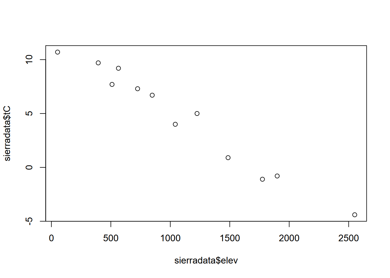
FIGURE 2.5: Temperature~Elevation
2.6.4.2 Read a data frame from a CSV
We’ll be looking at this more in the next chapter, but a common need is to read data from a spreadsheet stored in the CSV format. Normally, you’d have that stored with your project and can just specify the file name, but we’ll access CSVs from the igisci package. Since you have this installed, it will already be on your computer, but not in your project folder. The path to it can be derived using the system.file() function.
Reading a csv in readr (part of the tidyverse that we’ll be looking at in the next chapter) is done with read_csv(). We’ll use the DT::datatable for this because it lets you interactively scroll across the many variables, and this table is included as Figure 2.6.
library(readr)
csvPath <- system.file("extdata","TRI/TRI_2017_CA.csv", package="igisci")
TRI2017 <- read_csv(csvPath)DT::datatable(TRI2017, options=list(scrollX=T))FIGURE 2.6: TRI dataframe – DT datatable output
Note that we could have used the built-in read.csv function, but as you’ll see later, there are advantages of readr::read_csv so we should get in the habit of using that instead.
2.6.4.3 Reorganizing data frames
There are quite a few ways to reorganize your data in R, and we’ll learn other methods in the next chapter where we start using the tidyverse which make data abstraction and transformation much easier. For now, we’ll work with a simpler CSV I’ve prepared:
csvPath <- system.file("extdata","TRI/TRI_1987_BaySites.csv", package="igisci")
TRI87 <- read_csv(csvPath)
TRI87
## # A tibble: 335 × 9
## TRI_FACILITY_ID count FACILI…¹ COUNTY air_r…² fugit…³ stack…⁴ LATIT…⁵ LONGI…⁶
## <chr> <dbl> <chr> <chr> <dbl> <dbl> <dbl> <dbl> <dbl>
## 1 91002FRMND585BR 2 FORUM I… SAN M… 1423 1423 0 37.5 -122.
## 2 92052ZPMNF2970C 1 ZEP MFG… SANTA… 337 337 0 37.4 -122.
## 3 93117TLDYN3165P 2 TELEDYN… SANTA… 12600 12600 0 37.4 -122.
## 4 94002GTWSG477HA 2 MORGAN … SAN M… 18700 18700 0 37.5 -122.
## 5 94002SMPRD120SE 2 SEM PRO… SAN M… 1500 500 1000 37.5 -122.
## 6 94025HBLNN151CO 2 HEUBLEI… SAN M… 500 0 500 37.5 -122.
## 7 94025RYCHM300CO 10 TE CONN… SAN M… 144871 47562 97309 37.5 -122.
## 8 94025SNFRD990OB 1 SANFORD… SAN M… 9675 9675 0 37.5 -122.
## 9 94026BYPCK3575H 2 BAY PAC… SAN M… 80000 32000 48000 37.5 -122.
## 10 94026CDRSY3475E 2 CDR SYS… SAN M… 126800 0 126800 37.5 -122.
## # … with 325 more rows, and abbreviated variable names ¹FACILITY_NAME,
## # ²air_releases, ³fugitive_air, ⁴stack_air, ⁵LATITUDE, ⁶LONGITUDESort, Index, & Max/Min
One simple task is to sort data (numerically or by alphabetic order) such as a variable extracted as a vector.
head(sort(TRI87$air_releases))## [1] 2 5 5 7 9 10… or create an index vector of the order of our vector/variable…
index <- order(TRI87$air_releases)… where the index vector is just used to store the order of the TRI87$air_releases vector/variable; then we can use that index to display facilities in order of their air releases.
head(TRI87$FACILITY_NAME[index])## [1] "AIR PRODUCTS MANUFACTURING CORP"
## [2] "UNITED FIBERS"
## [3] "CLOROX MANUFACTURING CO"
## [4] "ICI AMERICAS INC WESTERN RESEARCH CENTER"
## [5] "UNION CARBIDE CORP"
## [6] "SCOTTS-SIERRA HORTICULTURAL PRODS CO INC"This is similar to filtering for a subset. We can also pull out individual values using functions like which.max to find the desired index value:
i_max <- which.max(TRI87$air_releases)
TRI87$FACILITY_NAME[i_max]   # was NUMMI at the time
## [1] "TESLA INC"2.6.5 Factors
Factors are vectors with predefined values, normally used for categorical data, and as R is a statistical language are frequently used to stratify data, such as defining groups for analysis of variance among those groups. They are built on an integer vector, and levels are the set of predefined values, which are commonly character data.
nut <- factor(c("almond", "walnut", "pecan", "almond"))
str(nut)   # note that levels will be in alphabetical order
## Factor w/ 3 levels "almond","pecan",..: 1 3 2 1typeof(nut)## [1] "integer"As always, there are multiple ways of doing things. Here’s an equivalent conversion that illustrates their relation to integers:
nutint <- c(1, 2, 3, 2) # equivalent conversion
nut <- factor(nutint, labels = c("almond", "pecan", "walnut"))
str(nut)
## Factor w/ 3 levels "almond","pecan",..: 1 2 3 22.6.5.1 Categorical Data and Factors
While character data might be seen as categorical (e.g. "urban", "agricultural", "forest" land covers), to be used as categorical variables they must be made into factors. So we have something to work with, we’ll generate some random memberships in one of three vegetation moisture categories using the sample() function:
veg_moisture_categories <- c("xeric", "mesic", "hydric")
veg_moisture_char <- sample(veg_moisture_categories, 42, replace = TRUE)
veg_moisture_fact <- factor(veg_moisture_char, levels = veg_moisture_categories)
veg_moisture_char
## [1] "xeric" "mesic" "hydric" "hydric" "xeric" "mesic" "xeric" "hydric"
## [9] "hydric" "xeric" "mesic" "hydric" "mesic" "mesic" "mesic" "mesic"
## [17] "hydric" "mesic" "xeric" "hydric" "hydric" "mesic" "mesic" "xeric"
## [25] "xeric" "hydric" "xeric" "mesic" "mesic" "hydric" "mesic" "xeric"
## [33] "mesic" "mesic" "xeric" "mesic" "hydric" "xeric" "hydric" "xeric"
## [41] "xeric" "mesic"veg_moisture_fact## [1] xeric mesic hydric hydric xeric mesic xeric hydric hydric xeric
## [11] mesic hydric mesic mesic mesic mesic hydric mesic xeric hydric
## [21] hydric mesic mesic xeric xeric hydric xeric mesic mesic hydric
## [31] mesic xeric mesic mesic xeric mesic hydric xeric hydric xeric
## [41] xeric mesic
## Levels: xeric mesic hydricTo make a categorical variable a factor:
nut <- c("almond", "walnut", "pecan", "almond")
farm <- c("organic", "conventional", "organic", "organic")
ag <- as.data.frame(cbind(nut, farm))
ag$nut <- factor(ag$nut)
ag$nut
## [1] almond walnut pecan almond
## Levels: almond pecan walnutFactor example
library(igisci)
sierraFeb$COUNTY <- factor(sierraFeb$COUNTY)
str(sierraFeb$COUNTY)
## Factor w/ 21 levels "Amador","Butte",..: 20 14 7 12 12 2 19 11 2 19 ...2.7 Accessors and subsetting
The use of accessors in R can be confusing but they’re very important to understand. An accessor is “a method for accessing data in an object usually an attribute of that object” (Brown (n.d.)), so a method for subsetting, and for R these are [], [[]], and $, but it can be confusing to know when you might use which one. There are good reasons to have these three types for code clarity, however you can also use [] with a bit of clumsiness for all purposes.
We’ve already been using these in this chapter and will continue to use them throughout the book. Let’s look at the various accessors and subsetting options:
2.7.1 [] Subsetting
You use this to get a subset of any R object, whether it be a vector, list, or data frame. For a vector, the subset might be defined by indices …
lats <- c(37.5,47.4,29.4,33.4)
str(lats[4])
## num 33.4str(lats[2:3])## num [1:2] 47.4 29.4str(letters[24:26])## chr [1:3] "x" "y" "z"… or a Boolean with TRUE or FALSE values representing which to keep or not.
str(lats[c(TRUE,FALSE,TRUE,TRUE)])## num [1:3] 37.5 29.4 33.4An initially surprising but very handy way of creating one of these is to reference the vector itself in a relational expression. The following returns the same as the above, with the purpose of selecting all lats that are less than 40:
str(lats[lats<40])## num [1:3] 37.5 29.4 33.4Getting one element from a data frame will return a data frame, in this case a data frame with just one variable. For columns especially, you might expect the result to be a vector, but it’s a data frame with just one variable. Note that you can use either the column number or the name of the variable.
str(cars)## 'data.frame': 50 obs. of 2 variables:
## $ speed: num 4 4 7 7 8 9 10 10 10 11 ...
## $ dist : num 2 10 4 22 16 10 18 26 34 17 ...str(cars[1])## 'data.frame': 50 obs. of 1 variable:
## $ speed: num 4 4 7 7 8 9 10 10 10 11 ...str(cars["speed"])## 'data.frame': 50 obs. of 1 variable:
## $ speed: num 4 4 7 7 8 9 10 10 10 11 ...Similarly, subsetting to get a single observation (a row of values) with the [n,] method returns a very small data frame, or can be used to create a subset of a range or selection of observations:
cars[1,]## speed dist
## 1 4 2cars[3:5,]## speed dist
## 3 7 4
## 4 7 22
## 5 8 16cars[cars["speed"]<10,]## speed dist
## 1 4 2
## 2 4 10
## 3 7 4
## 4 7 22
## 5 8 16
## 6 9 10Getting a data frame this way is very useful because many functions you’ll want to use require a data frame as input.
But sometimes you just want a vector. If you select an individual variable using the [,n] method, you’ll get one. You’ll want to assign it to a meaningful name like the original variable name. Note that you can either use the variable name or the variable column number:
dist <- cars[,"dist"] # or cars[,2]
dist
## [1] 2 10 4 22 16 10 18 26 34 17 28 14 20 24 28 26 34 34 46
## [20] 26 36 60 80 20 26 54 32 40 32 40 50 42 56 76 84 36 46 68
## [39] 32 48 52 56 64 66 54 70 92 93 120 852.7.2 [[]] The mysterious double bracket
Double brackets extract just one element, so just one value from a vector or one vector from a data frame. You’re going one step further into the structure.
str(cars[,"speed"])## num [1:50] 4 4 7 7 8 9 10 10 10 11 ...str(cars[["speed"]])## num [1:50] 4 4 7 7 8 9 10 10 10 11 ...Note that the str result is telling you that these are both simply vectors, not something like a data frame. Though uncommon, you can also use the index of variables instead of its name. Similar to the examples above, the variable can be specified either with the index (or column number) or the variable name. Since “speed” is the first variable in the cars data frame, these return the same thing:
str(cars[[1]])## num [1:50] 4 4 7 7 8 9 10 10 10 11 ...str(cars[["speed"]])## num [1:50] 4 4 7 7 8 9 10 10 10 11 ...2.7.3 $ Accessing a vector from a data frame
The $ accessor is really just a shortcut, but any shortcut reduces code and thus increases clarity, so it’s a good idea and this accessor is commonly used. Their only limitation is that you can’t use the integer indices, which would allow you to loop through a numerical sequence.
These accessor operations do the same thing:
cars$speed
cars[,"speed"]
cars[["speed"]]
## num [1:50] 4 4 7 7 8 9 10 10 10 11 ...Again, to contrast, the following accessor operations do the same thing – create a data frame:
sp1 <- cars[1] # gets the first variable, "speed"
sp2 <- cars["speed"]
str(sp1)
## 'data.frame': 50 obs. of 1 variable:
## $ speed: num 4 4 7 7 8 9 10 10 10 11 ...identical(sp1,sp2)## [1] TRUE2.8 Programming scripts in RStudio
Given the exploratory nature of the R language, we sometimes forget that it provides significant capabilities as a programming language where we can solve more complex problems by coding procedures and using logic to control the process and handle a range of possible scenarios.
Programming languages are used for a wide range of purposes, from developing operating systems built from low-level code to high-level scripting used to run existing functions in libraries. R and Python are commonly used for scripting, and you may be familiar with using arcpy to script ArcGIS geoprocessing tools. But whether low- or high-level, some common operational structures are used in all computer programming languages:
- Functions (defining your own)
- Conditional operations If a condition is true, do this.
- Loops
Common to all of these is an input in parentheses followed by what to do in braces:
- obj
<- function(input){process ending in an expression result} if(condition){process}if(condition){process} else {process}for(objectinlist){process}
The { } braces are only needed if the process goes past the first line, so for instance the following examples don’t need them (and actually some of the spaces aren’t necessary either, but I left them in for clarity):
a <- 2
f <- function(a) a*2
print(f(4))
if(a==3) print('yes') else print('no')
for(i in 1:5) print(i)
2.8.1 Functions you create
function(input){Do this and return the resulting expression}
The various packages that we’re installing, all those that aren’t purely data (like igisci), are built primarily of functions and perhaps most of those functions are written in R. Many of these simply make existing R functions work better or at least differently, often for a particular data science task common needed in a discipline or application area.
In geospatial environmental research for instance, we are often dealing with direction, for instance the movement of marine mammals who might be influenced by ship traffic. An agent-based model simulation of marine mammal movement might have the animal respond by shifting to the left or right, so we might want a turnLeft() or turnRight() function. Given the nature of circular data however, the code might be sufficiently complex to warrant writing a function that will make our main code easier to read:
turnright <- function(ang){(ang + 90) %% 360}Then in our code later on, after we’ve prepared some data …
id <- c("5A", "12D", "3B")
direction <- c(260, 270, 300)
whale <- dplyr::bind_cols(id = id,direction = direction) # better than cbind
whale
## # A tibble: 3 × 2
## id direction
## <chr> <dbl>
## 1 5A 260
## 2 12D 270
## 3 3B 300… we can call this function:
whale$direction <- turnright(whale$direction)
whale
## # A tibble: 3 × 2
## id direction
## <chr> <dbl>
## 1 5A 350
## 2 12D 0
## 3 3B 30Another function I found useful for our external data in igisci is to simplify the code needed to access the external data. I found I had to keep looking up the syntax for that task that we use a lot. It also makes the code difficult to read. Adding this function to the top of your code helps for both:
ex <- function(fnam){system.file("extdata",fnam,package="igisci")}Then our code that accesses data is greatly simplified, with read.csv calls looking a lot like reading data stored in our project folder. Where if we had fishdata.csv stored locally in our project folder, we might read it with …
read.csv("fishdata.csv")
… reading from the data package’s extdata folder looks pretty similar:
read.csv(ex("fishdata.csv"))
This simple function was so useful that it’s now included in the igisci package, so you can just call it with ex() if you have library(igisci) in your code.
Note on {}: You only really need the braces if you need more than one line of code in the function. The same will apply to the if..else and for programming structures we’ll look at next.
2.8.2 if else : Conditional operations
if (condition) {Do this} else {Do this other thing}
Probably not used as much in R for most users, as it’s mostly useful for building a new tool (or function) that needs to run as a complete operation. (But I found it essential in writing this book to create some outputs differently for the output to html than for the output to LaTeX for the pdf/book version.)
Common in coding is the need to be able to handle a variety of inputs and avoid errors. Here’s an admittedly trivial example of some short code that avoids an error:
getRatio <- function(x,y){
  if (y!=0){x/y} else {1e1000}
}

getRatio(5,0)
## [1] InfgetRatio(2,5)## [1] 0.4Note that the
else {needs to follow the close of theif (...) {...}section on the same line.
2.8.3 Loops
for(counterinlist){*Do something*}`
Loops are very common in traditional computer languages (in FORTRAN they were called Do Loops), but are not used as much in R due to its vectorization approach. But they still can be useful in some situations. The following is trivial but illustrates a simple loop that prints a series of results:
for(i in 1:10) print(paste(i, 1/i))## [1] "1 1"
## [1] "2 0.5"
## [1] "3 0.333333333333333"
## [1] "4 0.25"
## [1] "5 0.2"
## [1] "6 0.166666666666667"
## [1] "7 0.142857142857143"
## [1] "8 0.125"
## [1] "9 0.111111111111111"
## [1] "10 0.1"(Note the use of print above – this is one example where you have to use it.)
2.8.3.1 A for loop with an internal if..else
Here’s a more complex loop that builds river data for a map and profile that we’ll look at again in the visualization chapter. It also includes a conditional operation with if..else, embedded within the for loop (note the { } enclosures for each structure.)
x <- c(1000, 1100, 1300, 1500, 1600, 1800, 1900)
y <- c(500, 780, 820, 950, 1250, 1320, 1600)
elev <- c(0, 1, 2, 5, 25, 75, 150)
First a crude map from the xy coordinates (Figure 2.7):
plot(x,y,asp=1) + lines(x,y)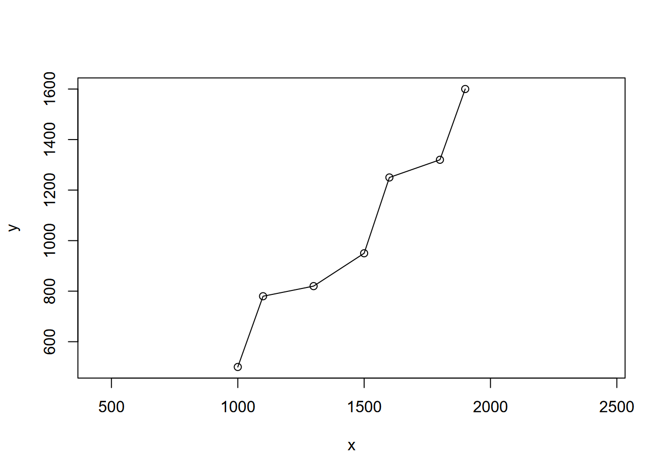
FIGURE 2.7: Crude river map using x y coordinates
## integer(0)Now we’ll use a loop to create a longitudinal graph by determining a cumulative longitudinal distance along the path of the river. You could look at it as straightening out the curves.
First we’ll need empty vectors to populate with the longitudinal profile data:
d <- double()      # creates an empty numeric vector
longd <- double()  # ("double" means double-precision floating point)
s <- double()
Then the for loop that goes through all of the points, but uses an if statement to assign an initial distance and longitudinal distance of zero, since the longitudinal profile data is just started and we don’t have a distance yet.
for(i in 1:length(x)){
  if(i==1){longd[i] <- 0; d[i] <- 0} else {
    d[i] <- sqrt((x[i]-x[i-1])^2 + (y[i]-y[i-1])^2)
    longd[i] <- longd[i-1] + d[i]
    s[i-1] <- (elev[i]-elev[i-1])/d[i]
    }
  }
There is no known slope for the last point (since we have no next point), so the last slope is assigned NA.
s[length(x)] <- NAThen we’ll create a data frame out of the vectors we just built, and then display the longitudinal profile (Figure 2.8).
riverData <- as.data.frame(cbind(x=x,y=y,elev=elev,d=d,longd=longd,s=s))
riverData
## x y elev d longd s
## 1 1000 500 0 0.0000 0.0000 0.003363364
## 2 1100 780 1 297.3214 297.3214 0.004902903
## 3 1300 820 2 203.9608 501.2822 0.012576654
## 4 1500 950 5 238.5372 739.8194 0.063245553
## 5 1600 1250 25 316.2278 1056.0471 0.235964589
## 6 1800 1320 75 211.8962 1267.9433 0.252252298
## 7 1900 1600 150 297.3214 1565.2647 NAplot(riverData$longd, riverData$elev) + lines(riverData$longd, riverData$elev)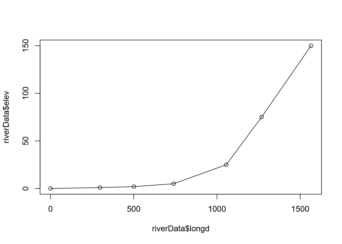
FIGURE 2.8: Longitudinal profile built from cumulative distances, and elevation
## integer(0)2.8.4 Subsetting with logic
We’ll use the 2022 USDOE fuel efficiency data to list all of the car lines with at least 50 miles to the gallon. Note the creation of a Boolean logical expression with an admittedly long variable ... >= 50; this will return TRUE or FALSE, so i will be a logical (Boolean) vector which can be used to subset a couple of variables which we’ll then paste together (using vectorization of course) to create a character string vector.
library(readxl)
fuelEff22 <- read_excel(ex("USDOE_FuelEfficiency2022.xlsx"))
i <- fuelEff22$`Hwy FE (Guide) - Conventional Fuel` >= 50
str(i)
## logi [1:394] FALSE FALSE FALSE FALSE FALSE FALSE ...efficientCars <- paste(fuelEff22$Division[i],fuelEff22$Carline[i])
str(efficientCars)## chr [1:9] "TOYOTA COROLLA HYBRID" "HYUNDAI MOTOR COMPANY Elantra Hybrid" ...efficientCars## [1] "TOYOTA COROLLA HYBRID"
## [2] "HYUNDAI MOTOR COMPANY Elantra Hybrid"
## [3] "HYUNDAI MOTOR COMPANY Elantra Hybrid Blue"
## [4] "TOYOTA PRIUS"
## [5] "TOYOTA PRIUS Eco"
## [6] "HYUNDAI MOTOR COMPANY Ioniq"
## [7] "HYUNDAI MOTOR COMPANY Ioniq Blue"
## [8] "HYUNDAI MOTOR COMPANY Sonata Hybrid"
## [9] "HYUNDAI MOTOR COMPANY Sonata Hybrid Blue"The which function allows us to do something similar, returning the indices of the variable or vector for which a condition TRI87$air_releases > 1e6 is TRUE. Then we can use that index to do the subset.
library(readr)
csvPath = system.file("extdata","TRI/TRI_1987_BaySites.csv", package="igisci")
TRI87 <- read_csv(csvPath)
i <- which(TRI87$air_releases > 1e6)
str(i)
## int [1:4] 85 96 127 328TRI87$FACILITY_NAME[i]## [1] "VALERO REFINING CO-CALI FORNIA BENICIA REFINERY"
## [2] "TESLA INC"
## [3] "TESORO REFINING & MARKETING CO LLC"
## [4] "HGST INC"The %in% operator is very useful when we have very specific items to select.
library(readr)
csvPath = system.file("extdata","TRI/TRI_1987_BaySites.csv", package="igisci")
TRI87 <- read_csv(csvPath)
i <- TRI87$COUNTY %in% c("NAPA","SONOMA")
TRI87$FACILITY_NAME[i]
## [1] "SAWYER OF NAPA"
## [2] "BERINGER VINEYARDS"
## [3] "CAL-WOOD DOOR INC"
## [4] "SOLA OPTICAL USA INC"
## [5] "KEYSIGHT TECHNOLOGIES INC"
## [6] "SANTA ROSA STAINLESS STEEL"
## [7] "OPTICAL COATING LABORATORY INC"
## [8] "MGM BRAKES"
## [9] "SEBASTIANI VINEYARDS INC, SONOMA CASK CELLARS"2.8.5 Apply functions
There are many apply functions in R, and they largely obviate the need for looping. For instance:
applyderives values at margins of rows and columns, e.g. to sum across rows or down columns [create the following in a newgeneric_methodsproject which you’ll use for a variety of generic methods]
# matrix apply – the same would apply to data frames
matrix12 <- 1:12
dim(matrix12) <- c(3,4)
rowsums <- apply(matrix12, 1, sum)
colsums <- apply(matrix12, 2, sum)
sum(rowsums)
## [1] 78sum(colsums)## [1] 78zero <- sum(rowsums) - sum(colsums)
matrix12## [,1] [,2] [,3] [,4]
## [1,] 1 4 7 10
## [2,] 2 5 8 11
## [3,] 3 6 9 12Apply functions satisfy one of the needs that spreadsheets are used for. Consider how often you use sum, mean or similar functions in Excel.
sapply
sapply applies functions to either:
- all elements of a vector – unary functions only
sapply(1:12, sqrt)## [1] 1.000000 1.414214 1.732051 2.000000 2.236068 2.449490 2.645751 2.828427
## [9] 3.000000 3.162278 3.316625 3.464102- or all variables of a data frame (not a matrix), where it works much like a column-based apply (since variables are columns) but more easily interpreted without the need of specifying columns with 2:
sapply(cars,mean) # same as apply(cars,2,mean)## speed dist
## 15.40 42.98temp02 <- c(10.7,9.7,7.7,9.2,7.3,6.7,4.0,5.0,0.9,-1.1,-0.8,-4.4)
temp03 <- c(13.1,11.4,9.4,10.9,8.9,8.4,6.7,7.6,2.8,1.6,1.2,-2.1)
sapply(as.data.frame(cbind(temp02,temp03)),mean) # has to be a data frame## temp02 temp03
## 4.575000 6.658333While various apply functions are in base R, the purrr package takes these further. See https://www.rstudio.com/resources/cheatsheets/ for more information on this and other packages in the RStudio/tidyverse world.
2.9 RStudio projects
So far, you’ve been using RStudio and it organizes your code and data into a project folder. You should familiarize yourself with where things are being saved and where you can find things. Start by seeing your working directory with :
getwd()When you create a new RStudio project with File/New Project..., it will set the working directory to the project folder where you create the project. (You can change the working directory with setwd() but I don’t recommend it.) The project folder is useful for keeping things organized and allowing you to use relative paths to your data and allow everything to be moved somewhere else and still work. The project file has the extension .Rproj and it will reside in the project folder. If you’ve saved any scripts (.R)or R Markdown (.Rmd) documents, they’ll also reside in the project folder; and if you’ve saved any data, or if you want to read any data without providing the full path or using the extdata access method, those data files (e.g. .csv) will be in that project folder. You can see your scripts, R Markdown documents and data files using the Files tab in the default lower right pane of RStudio.
RStudio projects are going to be the way we’ll want to work for the rest of this book, so you’ll often want to create new ones for particular data sets so things don’t get messy. And you may want to create data folders within your project folder, as we have in the igisci extdata folder, to keep things organized. Since we’re using our igisci package, this is less of an issue since at least input data aren’t stored in the project folder. However you’re going to be creating data, so you’ll want to manage your data in individual projects. You may want to start a new project for each data set, using File/New Project, and try to keep things organized (things can get messy fast!)
In this book, we’ll be making a lot of use of data provided for you from various data packages such as built-in data, palmerpenguins (Horst, Hill, and Gorman 2020), or igisci, but they correspond to specific research projects, such as Sierra Climate to which several data frames and spatial data apply. For this chapter, you can probably just use one project, but later you’ll find it useful to create separate projects for each data set – such as a sierra project and return to it every time it applies.
In that project, you’ll build a series of scripts, many of which you’ll re-use to develop new methods. When you’re working on your own project with your own data files, you should store these in a data folder inside the project folder. With the project folder as the default working directory, you can use relative paths and everything will work even if the project folder is moved. So for instance you can specify "data/mydata.csv" as the path to a csv of that name. You can still access package data, including extdata folders and files, but your processed and saved or imported data will reside with your project.
An absolute path to somewhere on your computer in contrast won’t work for anyone else trying to run your code; absolute paths should only be used for servers that other users have access to and URLs on the web.
2.9.1 R Markdown
An alternative to writing scripts is writing R Markdown documents, which includes both formatted text (such as you’re seeing in this book, like the italics just used above which was created using asterisks) and code chunks. R lends itself to running code in chunks, as opposed to creating complete tools that run all of the way through. This book is built from R Markdown documents organized in a bookdown structure, and most of the figures are created from R code chunks. There are also many good resources on writing R Markdown documents, including the very thorough R Markdown: The Definitive Guide (Xie, Allaire, and Grolemund 2019).
Exercises
Assign scalars for your name, city, state and zip code, and use paste() to combine them, and assign them to the object me. What is the class of me?
:::
Exercise 2.1 Knowing that trigonometric functions require angles (including azimuth directions) to be provided in radians, and that degrees can be converted into radians by dividing by 180 and multiplying that by pi, derive the sine of 30 degrees with an R expression. (Base R knows what pi is, so you can just use pi)
Exercise 2.2 If two sides of a right triangle on a map can be represented as \(dX\) and \(dY\) and the direct line path between them \(c\), and the coordinates of 2 points on a map might be given as \((x1,y1)\) and \((x2,y2)\), with \(dX=x2-x1\) and \(dY=y2-y1\), use the Pythagorean theorem to derive the distance between them and assign that expression to \(c\). Start by assigning the input scalars.
Exercise 2.3 You can create a vector uniform random numbers from 0 to 1 using runif(n=30) where n=30 says to make 30 of them. Use the round() function to round each of the values (it vectorizes them), and provide what you created and explain what happened.
Exercise 2.4 Create two vectors of 10 numbers each with the c() function, then assigning to x and y. Then plot(x,y), and provide the three lines of code you used to do the assignment and plot.
Exercise 2.5 Change your code from #5 so that one value is NA (entered simply as NA, no quotation marks), and derive the mean value for x. Then add ,na.rm=T to the parameters for mean(). Also do this for y. Describe your results and explain what happens.
Exercise 2.6 Create two sequences, a and b, with a all odd numbers from 1 to 99, b all even numbers from 2 to 100. Then derive c through vector division of b/a. Plot a and c together as a scatterplot.
Exercise 2.7 Build the sierradata data frame from the data at the top of the Matrices section, also given here:
temp <- c(10.7, 9.7,  7.7,  9.2,  7.3,  6.7,   4.0,  5.0,  0.9, -1.1, -0.8,-4.4)
elev <- c(52,   394,  510,  564,  725,  848,  1042, 1225, 1486, 1775, 1899, 2551)
lat <-  c(39.52,38.91,37.97,38.70,39.09,39.25,39.94,37.75,40.35,39.33,39.17,38.21)
Create a data frame from it using the same steps, and plot temp against latitude.
Exercise 2.8 From the sierradata matrix built with cbind(), derive colmeans using the mean parameter on the columns 2 for apply().
Exercise 2.9 Do the same thing with the sierra data data frame with sapply().