Chapter 3 Data Abstraction
Abstracting data from large data sets (or even small ones) is critical to data science. The most common first step to visualization is abstracting the data in a form that allows for the visualization goal in mind. If you’ve ever worked with data in spreadsheets, you commonly will be faced with some kind of data manipulation to create meaningful graphs, unless that spreadsheet is specifically designed for it, but then doing something else with the data is going to require some work.
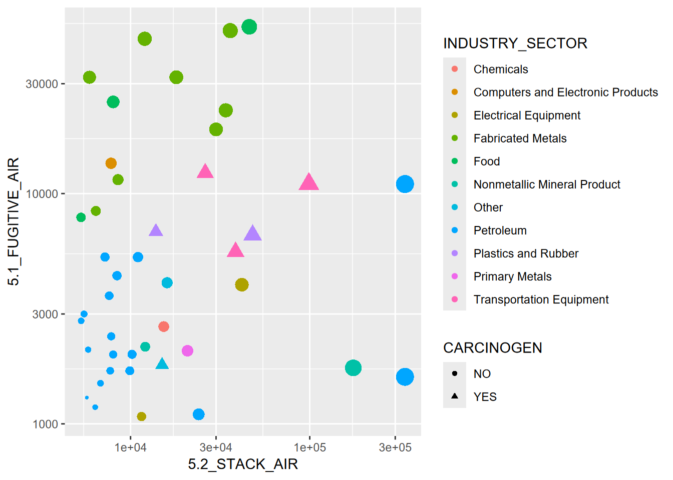
FIGURE 3.1: Visualization of some abstracted data from the EPA Toxic Release Inventory
Figure 3.1 started with abstracting some data from EPA’s Toxic Release Inventory (TRI) program, which holds data reported from a large number of facilities that must report either “stack” or “fugitive” air. Some of the abstraction had already happened when I used the EPA web site to download data for particular years and only in California. But there’s more we need to do, and we’ll want to use some dplyr functions to help with it.
At this point, we’ve learned the basics of working with the R language. From here we’ll want to explore how to analyze data, statistically, spatially, and temporally. One part of this is abstracting information from existing data sets by selecting variables and observations and summarizing their statistics.
In the previous chapter, we learned some abstraction methods in base R, such as selecting parts of data frames and applying some functions across the data frame. There’s a lot we can do with these methods, and we’ll continue to use them, but they can employ some fairly arcane language. There are many packages that extend R’s functionality, but some of the most important for data science can be found in the various packages of “The Tidyverse” (Wickham 2017), which has the philosophy of making data manipulation more intuitive.
We’ll start with dplyr, which includes an array of data manipulation tools, including select for selecting variables, filter for subsetting observations, summarize for reducing variables to summary statistics, typically stratified by groups, and mutate for creating new variables from mathematical expressions from existing variables. Some dplyr tools such as data joins we’ll look at later in the data transformation chapter.
3.1 The Tidyverse
The Tidyverse refers to a suite of R packages developed at RStudio (see https://rstudio.com and <https://r4ds.had.co.nz>) for facilitating data processing and analysis. While R itself is designed around exploratory data analysis, the Tidyverse takes it further. Some of the packages in the Tidyverse that are widely used are:
dplyr: data manipulation like a databasereadr: better methods for reading and writing rectangular datatidyr: reorganization methods that extend dplyr’s database capabilitiespurrr: expanded programming toolkit including enhanced “apply” methodstibble: improved data framestringr: string manipulation libraryggplot2: graphing system based on the grammar of graphics
In this chapter, we’ll be mostly exploring dplyr, with a few other
things thrown in like reading data frames with readr. For
simplicity, we can just include library(tidyverse) to get everything.
3.2 Tibbles
Tibbles are an improved type of data frame
- part of the Tidyverse
- serve the same purpose as a data frame, and all data frame operations work
Advantages
- display better
- can be composed of more complex objects like lists, etc.
- can be grouped
There multiple ways to create a tibble:
- Reading from a CSV using
read_csv(). Note the underscore, a function naming convention in the tidyverse. - Using
tibble()to either build from vectors or from scratch, or convert from a different type of data frame. - Using
tribble()to build in code from scratch. - Using various tidyverse functions that return tibbles.
3.2.1 Building a tibble from vectors
We’ll start by looking at a couple of built-in character vectors (there
are lots of things like this in R) - letters : lower case letters -
LETTERS : upper case letters’s also a LETTERS and lots of other
things like that in R)…
letters## [1] "a" "b" "c" "d" "e" "f" "g" "h" "i" "j" "k" "l" "m" "n" "o" "p" "q" "r" "s"
## [20] "t" "u" "v" "w" "x" "y" "z"LETTERS## [1] "A" "B" "C" "D" "E" "F" "G" "H" "I" "J" "K" "L" "M" "N" "O" "P" "Q" "R" "S"
## [20] "T" "U" "V" "W" "X" "Y" "Z"… then make a tibble of letters, LETTERS, and two random sets of
26 values, one normally distributed, the other uniform:
norm <- rnorm(26)
unif <- runif(26)
library(tidyverse)
tibble26 <- tibble(letters,LETTERS,norm,unif)
tibble26
## # A tibble: 26 × 4
## letters LETTERS norm unif
## <chr> <chr> <dbl> <dbl>
## 1 a A -0.433 0.670
## 2 b B -0.301 0.507
## 3 c C -0.753 0.0376
## 4 d D -1.32 0.578
## 5 e E -0.808 0.0170
## 6 f F -0.725 0.599
## 7 g G 1.58 0.369
## 8 h H 0.191 0.140
## 9 i I 0.937 0.574
## 10 j J -1.12 0.175
## # … with 16 more rows3.2.2 tribble
As long as you don’t let them multiply in your starship, the tribble method is a handy hard-coding way to create a tibble from scratch. You simply create the variable names with a series of entries starting with a tilde, then the data are entered one row at a time. If you line them all up in your code one row at a time, it’s easy to enter the data accurately (Table 3.1).
peaks <- tribble(
  ~peak, ~elev, ~longitude, ~latitude,
  "Mt. Whitney", 4421, -118.2, 36.5,
  "Mt. Elbert", 4401, -106.4, 39.1,
  "Mt. Hood", 3428, -121.7, 45.4,
  "Mt. Rainier", 4392, -121.8, 46.9)
knitr::kable(peaks, caption = 'Peaks tibble')| peak | elev | longitude | latitude |
|---|---|---|---|
| Mt. Whitney | 4421 | -118.2 | 36.5 |
| Mt. Elbert | 4401 | -106.4 | 39.1 |
| Mt. Hood | 3428 | -121.7 | 45.4 |
| Mt. Rainier | 4392 | -121.8 | 46.9 |
3.2.3 read_csv
The read_csv function does somewhat the same thing as read.csv in
base R, but creates a tibble instead of a data.frame, and has some other
properties we’ll look at below.
Note that the code below accesses data we’ll be using a lot, from EPA
Toxic Release Inventory (TRI) data. If you want to keep this data
organized in a separate project, you might consider creating a new
air_quality project. This is optional, and you can get by with
staying in one project since all of our data will be accessed from the
igisci package. But in your own work, you will find it useful to
create separate projects to keep things organized with your code and
data together.
library(tidyverse); library(igisci)
TRI87 <- read_csv(ex("TRI/TRI_1987_BaySites.csv"))
TRI87df <- read.csv(ex("TRI/TRI_1987_BaySites.csv"))
TRI87b <- tibble(TRI87df)
identical(TRI87, TRI87b)
## [1] FALSENote that they’re not identical. So what’s the difference between
read_csv and read.csv? Why would we use one over the other? Since
their names are so similar, you may accidentally choose one or the
other. Some things to consider:
- To use read_csv, you need to load the
readrortidyverselibrary, or usereadr::read_csv. - read.csv “fixes” some things and sometimes that might be desired:
problematic variable names like
MLY-TAVG-NORMALbecomeMLY.TAVG.NORMAL– but this may create problems if those original names are a standard designation. - With
read.csv, numbers stored as characters are converted to numbers: “01” becomes 1, “02” becomes 2, etc. - There are other known problems that read_csv avoids.
Recommendation: Use read_csv and write_csv.
Final note on tibbles: You can still just call tibbles “data frames”, since they are still data frames, and in this book we’ll follow that practice. For all intents and purposes, they’re just data frames.
3.3 Summarizing variable distributions
A simple statistical summary is very easy to do in R, and we’ll use
eucoak data in the igisci package from a study of comparative
runoff and erosion under Eucalyptus and oak canopies (Thompson, Davis, and Oliphant 2016). In this
study (Figure 3.2), we looked at the amount of runoff and erosion captured in Gerlach troughs on paired eucalyptus and oak sites in the San Francisco Bay
Area. You might consider creating a eucoak project, since we’ll be
referencing this data set in several places.
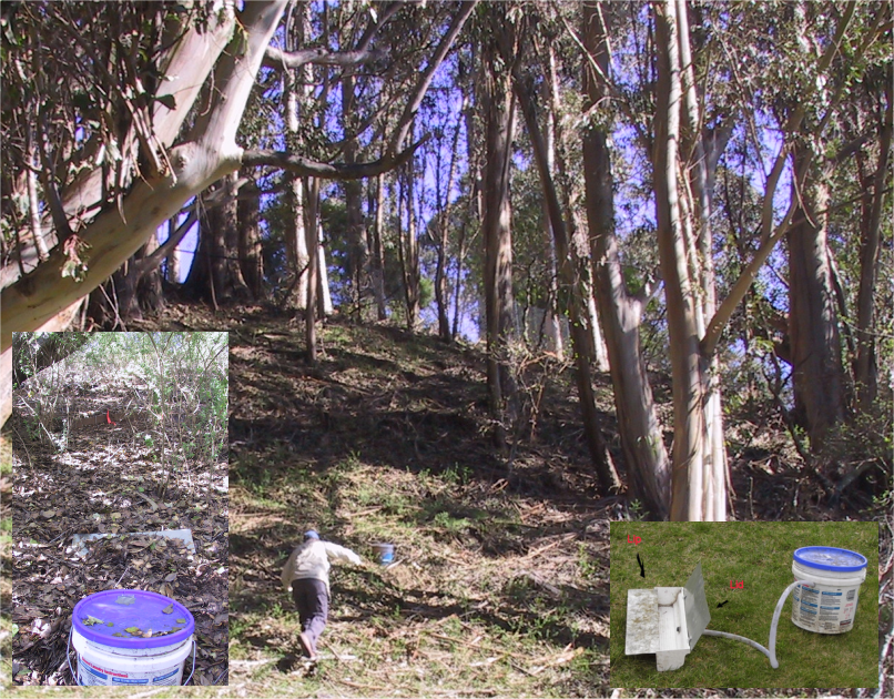
FIGURE 3.2: Euc-Oak paired plot runoff and erosion study
library(igisci)
summary(eucoakrainfallrunoffTDR)
## site site # date month
## Length:90 Min. :1.000 Length:90 Length:90
## Class :character 1st Qu.:2.000 Class :character Class :character
## Mode :character Median :4.000 Mode :character Mode :character
## Mean :4.422
## 3rd Qu.:6.000
## Max. :8.000
##
## rain_mm rain_oak rain_euc runoffL_oak
## Min. : 1.00 Min. : 1.00 Min. : 1.00 Min. : 0.000
## 1st Qu.:16.00 1st Qu.:16.00 1st Qu.:14.75 1st Qu.: 0.000
## Median :28.50 Median :30.50 Median :30.00 Median : 0.450
## Mean :37.99 Mean :35.08 Mean :34.60 Mean : 2.032
## 3rd Qu.:63.25 3rd Qu.:50.50 3rd Qu.:50.00 3rd Qu.: 2.800
## Max. :99.00 Max. :98.00 Max. :96.00 Max. :14.000
## NA's :18 NA's :2 NA's :2 NA's :5
## runoffL_euc slope_oak slope_euc aspect_oak
## Min. : 0.00 Min. : 9.00 Min. : 9.00 Min. :100.0
## 1st Qu.: 0.07 1st Qu.:12.00 1st Qu.:12.00 1st Qu.:143.0
## Median : 1.20 Median :24.50 Median :23.00 Median :189.0
## Mean : 2.45 Mean :21.62 Mean :19.34 Mean :181.9
## 3rd Qu.: 3.30 3rd Qu.:30.50 3rd Qu.:25.00 3rd Qu.:220.0
## Max. :16.00 Max. :32.00 Max. :31.00 Max. :264.0
## NA's :3
## aspect_euc surface_tension_oak surface_tension_euc
## Min. :106.0 Min. :37.40 Min. :28.51
## 1st Qu.:175.0 1st Qu.:72.75 1st Qu.:32.79
## Median :196.5 Median :72.75 Median :37.40
## Mean :191.2 Mean :68.35 Mean :43.11
## 3rd Qu.:224.0 3rd Qu.:72.75 3rd Qu.:56.41
## Max. :296.0 Max. :72.75 Max. :72.75
## NA's :22 NA's :22
## runoff_rainfall_ratio_oak runoff_rainfall_ratio_euc
## Min. :0.00000 Min. :0.000000
## 1st Qu.:0.00000 1st Qu.:0.003027
## Median :0.02046 Median :0.047619
## Mean :0.05357 Mean :0.065902
## 3rd Qu.:0.08485 3rd Qu.:0.083603
## Max. :0.42000 Max. :0.335652
## NA's :5 NA's :3In the summary output, how are character variables handled differently from numeric ones?
Remembering what we discussed in the previous chapter, consider the site variable (Figure 3.3), and in particular its Length. Looking at the table, what does that length represent?
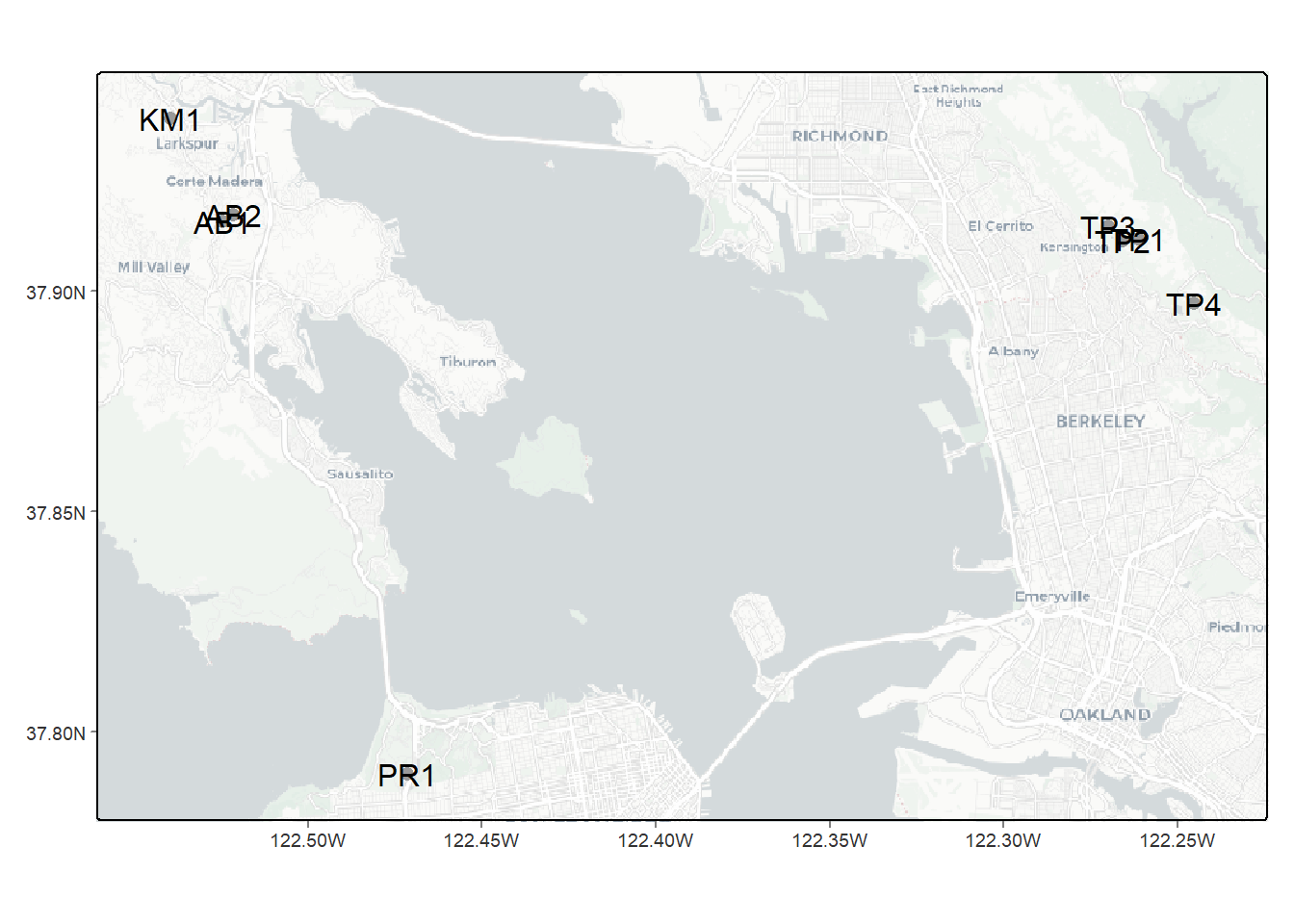
FIGURE 3.3: Eucalyptus/Oak paired site locations
There are a couple of ways of seeing what unique values exist in a
character variable like site which can be considered a categorical
variable (factor). Consider what these return:
unique(eucoakrainfallrunoffTDR$site)## [1] "AB1" "AB2" "KM1" "PR1" "TP1" "TP2" "TP3" "TP4"factor(eucoakrainfallrunoffTDR$site)## [1] AB1 AB1 AB1 AB1 AB1 AB1 AB1 AB1 AB1 AB1 AB1 AB1 AB2 AB2 AB2 AB2 AB2 AB2 AB2
## [20] AB2 AB2 AB2 AB2 AB2 KM1 KM1 KM1 KM1 KM1 KM1 KM1 KM1 KM1 KM1 KM1 KM1 PR1 PR1
## [39] PR1 PR1 PR1 PR1 PR1 PR1 PR1 PR1 TP1 TP1 TP1 TP1 TP1 TP1 TP1 TP1 TP1 TP1 TP1
## [58] TP2 TP2 TP2 TP2 TP2 TP2 TP2 TP2 TP2 TP2 TP2 TP3 TP3 TP3 TP3 TP3 TP3 TP3 TP3
## [77] TP3 TP3 TP3 TP4 TP4 TP4 TP4 TP4 TP4 TP4 TP4 TP4 TP4 TP4
## Levels: AB1 AB2 KM1 PR1 TP1 TP2 TP3 TP43.3.1 Stratifying variables by site using a Tukey box plot
A good way to look at variable distributions stratified by a sample site factor is the Tukey box plot (Figure 3.4). We’ll be looking more at this and other visualization methods in the next chapter.
ggplot(data = eucoakrainfallrunoffTDR) + geom_boxplot(mapping = aes(x=site, y=runoffL_euc))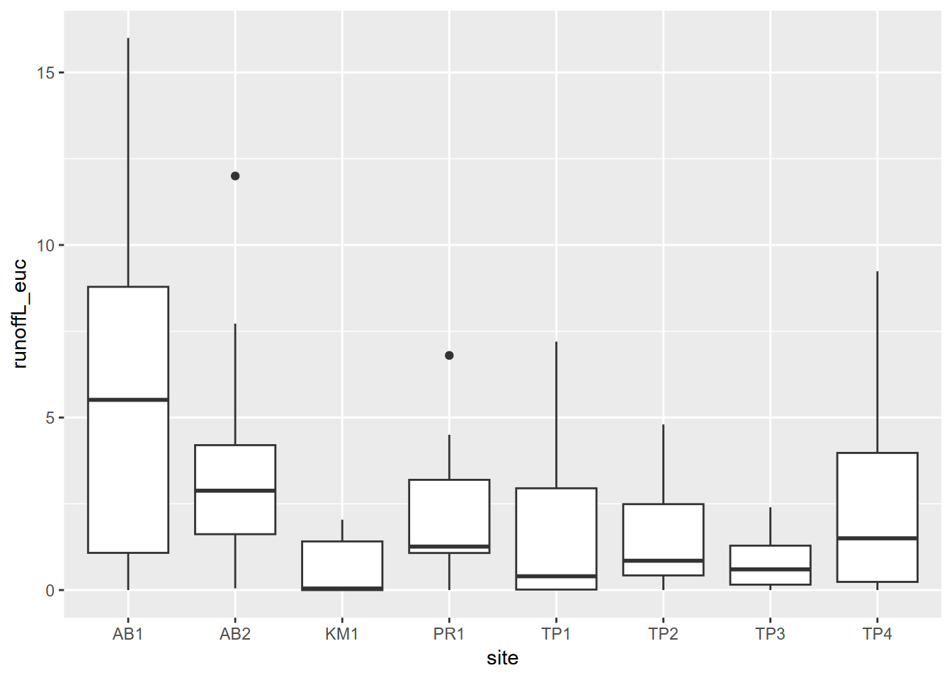
FIGURE 3.4: Tukey boxplot of runoff under Eucalyptus canopy
3.4 Database operations with dplyr
As part of exploring our data, we’ll typically simplify or reduce it for our purposes. The following methods are quickly discovered to be essential as part of exploring and analyzing data.
- select rows using logic, such as population > 10000, with
filter - select variable columns you want to retain with
select - add new variables and assign their values with
mutate - sort rows based on a a field with
arrange - summarize by group
3.4.1 Select, mutate, and the pipe
\index{“%>%”}The pipe %>%: Read %>% as “and then…” This is bigger than it
sounds and opens up a lot of possibilities.
See example below, and observe how the expression becomes several lines long. In the process, we’ll see examples of new variables with mutate and selecting (and in the process ordering) variables (Table 3.2).
runoff <- eucoakrainfallrunoffTDR %>%
  mutate(Date = as.Date(date,"%m/%d/%Y"),
         rain_subcanopy = (rain_oak + rain_euc)/2) %>%
  dplyr::select(site, Date, rain_mm, rain_subcanopy,
         runoffL_oak, runoffL_euc, slope_oak, slope_euc)
knitr::kable(head(runoff), caption = 'EucOak data reorganized a bit, first 6')| site | Date | rain_mm | rain_subcanopy | runoffL_oak | runoffL_euc | slope_oak | slope_euc |
|---|---|---|---|---|---|---|---|
| AB1 | 2006-11-08 | 29 | 29.0 | 4.7900 | 6.70000 | 32 | 31 |
| AB1 | 2006-11-12 | 22 | 18.5 | 3.2000 | 4.30000 | 32 | 31 |
| AB1 | 2006-11-29 | 85 | 65.0 | 9.7000 | 16.00000 | 32 | 31 |
| AB1 | 2006-12-12 | 82 | 87.5 | 14.0000 | 14.20000 | 32 | 31 |
| AB1 | 2006-12-28 | 43 | 54.0 | 9.7472 | 4.32532 | 32 | 31 |
| AB1 | 2007-01-29 | 7 | 54.0 | 1.4000 | 0.00000 | 32 | 31 |
Another way of thinking of the pipe that is very useful is that whatever goes before it becomes the first parameter for any functions that follow. So in the example above:
- The parameter
eucoakrainfallrunoffTDRbecomes the first formutate(), then - The result of the
mutate()becomes the first parameter fordplyr::select()
To just rename a variable, use
renameinstead ofmutate. It will stay in position.
3.4.1.1 Review: creating penguins from penguins_raw
To review some of these methods, it’s useful to consider how the penguins data frame was created from the more complex penguins_raw data frame, both of which are part of the palmerpenguins package (Horst, Hill, and Gorman (2020)). First let’s look at palmerpenguins::penguins_raw:
library(palmerpenguins)
library(tidyverse)
library(lubridate)
summary(penguins_raw)
## studyName Sample Number Species Region
## Length:344 Min. : 1.00 Length:344 Length:344
## Class :character 1st Qu.: 29.00 Class :character Class :character
## Mode :character Median : 58.00 Mode :character Mode :character
## Mean : 63.15
## 3rd Qu.: 95.25
## Max. :152.00
##
## Island Stage Individual ID Clutch Completion
## Length:344 Length:344 Length:344 Length:344
## Class :character Class :character Class :character Class :character
## Mode :character Mode :character Mode :character Mode :character
##
##
##
##
## Date Egg Culmen Length (mm) Culmen Depth (mm) Flipper Length (mm)
## Min. :2007-11-09 Min. :32.10 Min. :13.10 Min. :172.0
## 1st Qu.:2007-11-28 1st Qu.:39.23 1st Qu.:15.60 1st Qu.:190.0
## Median :2008-11-09 Median :44.45 Median :17.30 Median :197.0
## Mean :2008-11-27 Mean :43.92 Mean :17.15 Mean :200.9
## 3rd Qu.:2009-11-16 3rd Qu.:48.50 3rd Qu.:18.70 3rd Qu.:213.0
## Max. :2009-12-01 Max. :59.60 Max. :21.50 Max. :231.0
## NA's :2 NA's :2 NA's :2
## Body Mass (g) Sex Delta 15 N (o/oo) Delta 13 C (o/oo)
## Min. :2700 Length:344 Min. : 7.632 Min. :-27.02
## 1st Qu.:3550 Class :character 1st Qu.: 8.300 1st Qu.:-26.32
## Median :4050 Mode :character Median : 8.652 Median :-25.83
## Mean :4202 Mean : 8.733 Mean :-25.69
## 3rd Qu.:4750 3rd Qu.: 9.172 3rd Qu.:-25.06
## Max. :6300 Max. :10.025 Max. :-23.79
## NA's :2 NA's :14 NA's :13
## Comments
## Length:344
## Class :character
## Mode :character
##
##
##
## Now let’s create the simpler penguins data frame. We’ll use rename for a couple, but most variables required mutation, to manipulate strings (we’ll get to that later), create factors, or convert to integers. And we’ll rename some variables to avoid using backticks.
penguins <- penguins_raw %>%
  rename(bill_length_mm = `Culmen Length (mm)`,
         bill_depth_mm = `Culmen Depth (mm)`) %>%
  mutate(species = factor(word(Species)),
         island = factor(Island),
         flipper_length_mm = as.integer(`Flipper Length (mm)`),
         body_mass_g = as.integer(`Body Mass (g)`),
         sex = factor(str_to_lower(Sex)),
         year = as.integer(year(ymd(`Date Egg`)))) %>%
  dplyr::select(species, island, bill_length_mm, bill_depth_mm,
                flipper_length_mm, body_mass_g, sex, year)
summary(penguins)
## species island bill_length_mm bill_depth_mm
## Adelie :152 Biscoe :168 Min. :32.10 Min. :13.10
## Chinstrap: 68 Dream :124 1st Qu.:39.23 1st Qu.:15.60
## Gentoo :124 Torgersen: 52 Median :44.45 Median :17.30
## Mean :43.92 Mean :17.15
## 3rd Qu.:48.50 3rd Qu.:18.70
## Max. :59.60 Max. :21.50
## NA's :2 NA's :2
## flipper_length_mm body_mass_g sex year
## Min. :172.0 Min. :2700 female:165 Min. :2007
## 1st Qu.:190.0 1st Qu.:3550 male :168 1st Qu.:2007
## Median :197.0 Median :4050 NA's : 11 Median :2008
## Mean :200.9 Mean :4202 Mean :2008
## 3rd Qu.:213.0 3rd Qu.:4750 3rd Qu.:2009
## Max. :231.0 Max. :6300 Max. :2009
## NA's :2 NA's :2Unfortunately, they don’t end up as exactly identical, though all of the variables are identical as vectors:
identical(penguins, palmerpenguins::penguins)## [1] FALSE3.4.1.2 Helper functions for dplyr::select()
In the select() example above, we listed all of the variables, but there are a variety of helper functions for using logic to specify which variables to select:
contains("_")or any substring of interest in the variable name- `starts_with(“runoff”)
ends_with("euc")everything()matches()a regular expressionnum_range("x",1:5)for the common situation where a series of variable names combine a string and a numberone_of(myList)for when you have a group of variable names- range of variable: e.g.
runoffL_oak:slope_euccould have followedrain_subcanopyabove - all but (-): preface a variable or a set of variable names with - to select all others
3.4.2 filter
filter lets you select observations that meet criteria, similar to an SQL WHERE clause (Table 3.3).
runoff2007 <- runoff %>%
  filter(Date >= as.Date("04/01/2007", "%m/%d/%Y"))
knitr::kable(runoff2007, caption = 'Date-filtered EucOak data')| site | Date | rain_mm | rain_subcanopy | runoffL_oak | runoffL_euc | slope_oak | slope_euc |
|---|---|---|---|---|---|---|---|
| AB1 | 2007-04-23 | NA | 33.5 | 6.94488 | 9.19892 | 32.0 | 31 |
| AB1 | 2007-05-05 | NA | 31.0 | 6.33568 | 7.43224 | 32.0 | 31 |
| AB2 | 2007-04-23 | 23 | 35.5 | 4.32000 | 2.88000 | 24.0 | 25 |
| AB2 | 2007-05-05 | 11 | 25.5 | 4.98000 | 3.30000 | 24.0 | 25 |
| KM1 | 2007-04-23 | NA | 37.0 | 1.56000 | 2.04000 | 30.5 | 25 |
| KM1 | 2007-05-05 | 28 | 22.0 | 1.32000 | 1.32000 | 30.5 | 25 |
| PR1 | 2007-04-23 | NA | 31.5 | NA | 1.32000 | 27.0 | 23 |
| PR1 | 2007-05-05 | NA | 11.5 | 0.00000 | 1.20000 | 27.0 | 23 |
| TP1 | 2007-04-24 | 32 | 25.0 | 0.52500 | 0.40000 | 9.0 | 9 |
| TP1 | 2007-05-07 | 12 | 13.0 | 0.15000 | 0.60000 | 9.0 | 9 |
| TP2 | 2007-04-24 | 19 | 32.5 | 0.00000 | 2.28000 | 12.0 | 10 |
| TP2 | 2007-05-07 | 7 | 14.0 | 0.53000 | 0.74000 | 12.0 | 10 |
| TP3 | 2007-04-24 | 14 | 26.5 | 0.17500 | 1.70000 | 25.0 | 18 |
| TP3 | 2007-05-07 | 3 | 10.0 | 0.15000 | 0.60000 | 25.0 | 18 |
| TP4 | 2007-04-24 | 20 | 32.0 | 0.00000 | 1.80000 | 12.0 | 12 |
| TP4 | 2007-05-07 | 7 | 14.0 | 0.00000 | 1.50000 | 12.0 | 12 |
3.4.2.1 Filtering out NA with !is.na
Here’s a really important one. There are many times you need to avoid NAs. We thus commonly see summary statistics using na.rm = TRUE in order to ignore NAs when calculating a statistic like mean.
To simply filter out NAs from a vector or a variable use a filter:
feb_filt <- feb_s %>% filter(!is.na(TEMP))
3.4.3 Writing a data frame to a csv
Let’s say you have created a data frame, maybe with read_csv
runoff20062007 <- read_csv(ex("eucoak/eucoakrainfallrunoffTDR.csv"))
Then you do some processing to change it, maybe adding variables, reorganizing, etc., and you want to write out your new eucoak, so you just need to use write_csv
write_csv(eucoak, "data/tidy_eucoak.csv")
Note the use of a data folder
data: Remember that your default workspace (wdfor working directory) is where your project file resides (check what it is withgetwd()), so by default you’re saving things in that wd. To keep things organized the above code is placing data in a data folder within the wd.
3.4.4 Summarize by group
You’ll find that you need to use this all the time with real data. Let’s say you have a bunch of data where some categorical variable is defining a grouping, like our site field in the eucoak data. We’d like to just create average slope, rainfall, and runoff for each site. Note that it involves two steps, first defining which field defines the group, then the various summary statistics we’d like to store. In this case all of the slopes under oak remain the same for a given site – it’s a site characteristic – and the same applies to the euc site, so we can just grab the first value (mean would have also worked of course) (Table 3.4).
eucoakSiteAvg <- runoff %>%
  group_by(site) %>%
  summarize(
    rain = mean(rain_mm, na.rm = TRUE),
    rain_subcanopy = mean(rain_subcanopy, na.rm = TRUE),
    runoffL_oak = mean(runoffL_oak, na.rm = TRUE),
    runoffL_euc = mean(runoffL_euc, na.rm = TRUE),
    slope_oak = first(slope_oak),
    slope_euc = first(slope_euc)
  )
knitr::kable(eucoakSiteAvg, caption="EucOak data summarized by site")| site | rain | rain_subcanopy | runoffL_oak | runoffL_euc | slope_oak | slope_euc |
|---|---|---|---|---|---|---|
| AB1 | 48.37500 | 43.08333 | 6.8018364 | 6.0265233 | 32.0 | 31 |
| AB2 | 34.08333 | 35.37500 | 4.9113636 | 3.6545455 | 24.0 | 25 |
| KM1 | 48.00000 | 36.12500 | 1.9362500 | 0.5925000 | 30.5 | 25 |
| PR1 | 56.50000 | 37.56250 | 0.4585714 | 2.3100000 | 27.0 | 23 |
| TP1 | 38.36364 | 30.04545 | 0.8772727 | 1.6572727 | 9.0 | 9 |
| TP2 | 34.33333 | 32.86364 | 0.0954545 | 1.5254545 | 12.0 | 10 |
| TP3 | 32.09091 | 27.77273 | 0.3813636 | 0.8154545 | 25.0 | 18 |
| TP4 | 32.54545 | 35.72727 | 0.2309091 | 2.8259091 | 12.0 | 12 |
Summarizing by group with TRI data
library(igisci)
TRI_BySite <- read_csv(ex("TRI/TRI_2017_CA.csv")) %>%
  mutate(all_air = `5.1_FUGITIVE_AIR` + `5.2_STACK_AIR`) %>%
  filter(all_air > 0) %>%
  group_by(FACILITY_NAME) %>%
  summarize(
    FACILITY_NAME = first(FACILITY_NAME),
    air_releases = sum(all_air, na.rm = TRUE),
    mean_fugitive = mean(`5.1_FUGITIVE_AIR`, na.rm = TRUE),
    LATITUDE = first(LATITUDE), LONGITUDE = first(LONGITUDE))
3.4.5 Count
Count is a simple variant on summarize by group, since the only statistic is the count of events.
tidy_eucoak %>% count(tree)## # A tibble: 2 × 2
## tree n
## <chr> <int>
## 1 euc 90
## 2 oak 90Another way is to use n():
tidy_eucoak %>%
  group_by(tree) %>%
  summarize(n = n())
## # A tibble: 2 × 2
## tree n
## <chr> <int>
## 1 euc 90
## 2 oak 903.4.6 Sorting after summarizing
Using the marine debris data from the Marine Debris Monitoring and Assessment Project (Marine Debris Program, n.d.), we can use arrange to sort by latitude, so we can see the beaches from south to north along the Pacific coast.
shorelineLatLong <- ConcentrationReport %>%
  group_by(`Shoreline Name`) %>%
  summarize(
    latitude = mean((`Latitude Start`+`Latitude End`)/2),
    longitude = mean((`Longitude Start`+`Longitude End`)/2)
  ) %>%
  arrange(latitude)
shorelineLatLong
## # A tibble: 38 × 3
## `Shoreline Name` latitude longitude
## <chr> <dbl> <dbl>
## 1 Aimee Arvidson 33.6 -118.
## 2 Balboa Pier #2 33.6 -118.
## 3 Bolsa Chica 33.7 -118.
## 4 Junipero Beach 33.8 -118.
## 5 Malaga Cove 33.8 -118.
## 6 Zuma Beach, Malibu 34.0 -119.
## 7 Zuma Beach 34.0 -119.
## 8 Will Rodgers 34.0 -119.
## 9 Carbon Beach 34.0 -119.
## 10 Nicholas Canyon 34.0 -119.
## # … with 28 more rows3.4.7 The dot operator
The dot “.” operator derives from UNIX syntax, and refers to “here”.
- For accessing files in the current folder, the path is “./filename”
A similar specification is used in piped sequences
- The advantage of the pipe is you don’t have to keep referencing the data frame.
- The dot is then used to connect to items inside the data frame
TRI87 <- read_csv(ex("TRI/TRI_1987_BaySites.csv"))
stackrate <- TRI87 %>%
  mutate(stackrate = stack_air/air_releases) %>%
  .$stackrate
head(stackrate)
## [1] 0.0000000 0.0000000 0.0000000 0.0000000 0.6666667 1.00000003.5 String Abstraction
Character string manipulation is surprisingly critical to data analysis, and so the stringr package was developed to provide a wider array of string processing tools than what is in base R, including functions for detecting matches, subsetting strings, managing lengths, replacing substrings with other text, and joining, splitting, and sorting strings.
We’ll look at some of the stringr functions, but a good way to learn about the wide array of functions is through the cheat sheet that can be downloaded from https://www.rstudio.com/resources/cheatsheets/
3.5.1 Detecting matches
These functions look for patterns within existing strings which can then be used subset observations based on those patterns.
str_detectdetects patterns in a string, returns true or false if detectedstr_locatedetects patterns in a string, returns start and end position if detected, or NA if notstr_whichreturns the indices of strings that match a patternstr_countcounts the number of matches in each string
str_detect(fruit,"qu")## [1] FALSE FALSE FALSE FALSE FALSE FALSE FALSE FALSE FALSE FALSE FALSE FALSE
## [13] FALSE FALSE FALSE FALSE FALSE FALSE FALSE FALSE FALSE FALSE FALSE FALSE
## [25] FALSE FALSE FALSE FALSE FALSE FALSE FALSE FALSE FALSE FALSE FALSE FALSE
## [37] FALSE FALSE FALSE FALSE FALSE FALSE TRUE FALSE FALSE TRUE FALSE FALSE
## [49] FALSE FALSE FALSE FALSE FALSE FALSE FALSE FALSE FALSE FALSE FALSE FALSE
## [61] FALSE FALSE FALSE FALSE FALSE FALSE TRUE FALSE FALSE FALSE FALSE FALSE
## [73] FALSE FALSE FALSE FALSE FALSE FALSE FALSE FALSEfruit[str_detect(fruit,"qu")]## [1] "kumquat" "loquat" "quince"tail(str_locate(fruit, "qu"),15)## start end
## [66,] NA NA
## [67,] 1 2
## [68,] NA NA
## [69,] NA NA
## [70,] NA NA
## [71,] NA NA
## [72,] NA NA
## [73,] NA NA
## [74,] NA NA
## [75,] NA NA
## [76,] NA NA
## [77,] NA NA
## [78,] NA NA
## [79,] NA NA
## [80,] NA NAstr_which(fruit, "qu")## [1] 43 46 67fruit[str_which(fruit,"qu")]## [1] "kumquat" "loquat" "quince"str_count(fruit,"qu")## [1] 0 0 0 0 0 0 0 0 0 0 0 0 0 0 0 0 0 0 0 0 0 0 0 0 0 0 0 0 0 0 0 0 0 0 0 0 0 0
## [39] 0 0 0 0 1 0 0 1 0 0 0 0 0 0 0 0 0 0 0 0 0 0 0 0 0 0 0 0 1 0 0 0 0 0 0 0 0 0
## [77] 0 0 0 03.5.2 Subsetting Strings
Subsetting in this case includes its normal use of abstracting the observations specified by a match (similar to a filter for data frames), or just a specified part of a string specified by start and end character positions, or the part of the string that matches an expression.
str_subextracts a part of a string from a start to and end character positionstr_subsetreturns the strings that contain a pattern matchstr_extractreturns the first (or ifstr_extract_allthen all matches) pattern matchesstr_matchreturns the first (or_all) pattern match as a matrixstr_removeremoves a specific substring (not on the cheat sheet, but handy)
qfruit <- str_subset(fruit, "q")
qfruit
## [1] "kumquat" "loquat" "quince"str_sub(qfruit,1,2)## [1] "ku" "lo" "qu"str_sub("94132",1,2)## [1] "94"str_extract(qfruit,"[aeiou]")## [1] "u" "o" "u"str_remove(str_subset(fruit,"fruit"), "fruit")## [1] "bread" "dragon" "grape" "jack" "kiwi " "passion" "star "
## [8] "ugli "3.5.3 String Length
The length of strings is often useful in an analysis process, either just knowing the length as an integer, or purposefully increasing or reducing it.
str_lengthsimply returns the length of the string as an integerstr_padadds a specified character (typically a space ” “) to either end of a stringstr_trimremoves whitespace from the either end of a string
qfruit <- str_subset(fruit,"q")
qfruit
## [1] "kumquat" "loquat" "quince"str_length(qfruit)## [1] 7 6 6name <- "Inigo Montoya"
str_length(name)## [1] 13firstname <- str_sub(name,1,str_locate(name," ")[1]-1)
firstname## [1] "Inigo"lastname <- str_sub(name,str_locate(name," ")[1]+1,str_length(name))
lastname## [1] "Montoya"str_pad(qfruit,10,"both")## [1] " kumquat " " loquat " " quince "str_trim(str_pad(qfruit,10,"both"),"both")## [1] "kumquat" "loquat" "quince"3.5.4 Replacing substrings with other text (“mutating” strings)
These methods range from converting case to replace substrings.
str_to_lowerconverts strings to lower casestr_to_upperconverts strings to upper casestr_to_titlecapitalizes strings (makes the first character of each word upper case)str_suba special use of this function to replace substrings with a specified stringstr_replacereplaces the first matched pattern (or all withstr_replace_all) with a specified string
str_to_lower(name)## [1] "inigo montoya"str_to_upper(name)## [1] "INIGO MONTOYA"str_to_title("for whom the bell tolls")## [1] "For Whom The Bell Tolls"str_sub(name,1,str_locate(name," ")-1) <- "Diego"
str_replace(qfruit,"q","z")## [1] "kumzuat" "lozuat" "zuince"3.5.5 Concatenating and splitting
One very common string function is that to concatenate strings, and somewhat less common though useful is splitting them using a key separator like space, comma, or line end. One use of using str_c in the example below is to create a comparable join field based on a numeric character string that might need a zero or something at the left or right.
str_cThepaste()function in base R will work but you might want the default separator setting to be “” (as doespaste0()) instead of ” “, sostr_cis justpastewith a default”” separator, but you can also use ” “.str_splitsplits a string into parts based upon the detection of a specified separator like space, comma, or line end. However this ends up creating a list, which can be confusing to use. If you’re wanting to access a particular member of a list of words, thewordfunction is easier:wordlets you pick the first, second, or nth word in a string of words.
library(stringr)
phrase <- str_c("for","whom","the","bell","tolls",sep=" ")
phrase
## [1] "for whom the bell tolls"str_split(phrase, " ")## [[1]]
## [1] "for" "whom" "the" "bell" "tolls"word(phrase,4)## [1] "bell"… and of course, these methods can all be vectorized:
sentences[1:4]## [1] "The birch canoe slid on the smooth planks."
## [2] "Glue the sheet to the dark blue background."
## [3] "It's easy to tell the depth of a well."
## [4] "These days a chicken leg is a rare dish."word(sentences[1:4],2)## [1] "birch" "the" "easy" "days"Example of str_c use to modify a variable needed for a join:
csvPath <- system.file("extdata","CA/CA_MdInc.csv",package="igisci")
CA_MdInc <- read_csv(csvPath)
join_id <- str_c("0",CA_MdInc$NAME)
# could also use str_pad(CA_MdInc$NAME,1,side="left",pad="0")
head(CA_MdInc)
## # A tibble: 6 × 3
## trID NAME HHinc2016
## <dbl> <dbl> <dbl>
## 1 6001400100 60014001 177417
## 2 6001400200 60014002 153125
## 3 6001400300 60014003 85313
## 4 6001400400 60014004 99539
## 5 6001400500 60014005 83650
## 6 6001400600 60014006 61597head(join_id)## [1] "060014001" "060014002" "060014003" "060014004" "060014005" "060014006"3.6 Dates and times with lubridate
Simply stated, the lubridate package just makes it easier to work with dates and times. Dates and times are more difficult to work with than numbers and character strings, which is why lubridate was developed. The lubridate package is excellent at detecting and reading in dates and times – it can “parse” many forms. Spend some time to make sure you know how to use it. We’ll be using dates and times a lot, since many data sets include time stamps. See the cheat sheet for more information but the following examples may demonstrate that it’s pretty easy to use, and does a good job of making your job easier.
library(lubridate)
dmy("20 September 2020")
## [1] "2020-09-20"dmy_hm("20 September 2020 10:45")## [1] "2020-09-20 10:45:00 UTC"mdy_hms("September 20, 2020 10:48")## [1] "2020-09-20 20:10:48 UTC"mdy_hm("9/20/20 10:50")## [1] "2020-09-20 10:50:00 UTC"mdy("9.20.20")## [1] "2020-09-20"start704 <- dmy_hm("24 August 2020 16:00")
end704 <- mdy_hm("12/18/2020 4:45 pm")
year(start704)## [1] 2020month(start704)## [1] 8day(end704)## [1] 18hour(end704)## [1] 16end704-start704## Time difference of 116.0312 daysas_date(end704)## [1] "2020-12-18"hms::as_hms(end704)## 16:45:00You will find that dates are typically displayed as yyyy-mm-dd, e.g. “2020-09-20” above. You can display them other ways of course, but it’s useful to write dates this way since they sort better, with the highest order coming first.
For obvious reasons, we’ll use
lubridatea lot when we get to time series.
3.7 Calling functions explicitly with ::
Sometimes you need to specify the package and function name this way, for instance if more than one package has a function of the same name. You can also use this method to call a function without having loaded its library. Due to multiple packages having certain common names (like “select”), it’s common to use this syntax, and you’ll find that we’ll use dplyr::select(...) throughout this book.
Exercises
Exercise 3.1 Create a tibble with 20 rows of two variables norm and unif with norm created with rnorm() and unif created with runif().
Exercise 3.2 Read in “TRI/TRI_2017_CA.csv” in two ways, as a normal data frame assigned to df and as a tibble assigned to tbl. What field names result for what’s listed in the CSV as 5.1_FUGITIVE_AIR?
Exercise 3.3 Use the summary function to investigate the variables in either the data.frame or tibble you just created. What type of field and what values are assigned to BIA_CODE?
Exercise 3.4 Create a boxplot of body_mass_g by species from the penguins data frame in the palmerpenguins package (Horst, Hill, and Gorman 2020). Access the data with data(package = ‘palmerpenguins’), and also remember library(ggplot2) or library(tidyverse).
Exercise 3.5 Use select, mutate, and the pipe to create a penguinMass tibble where the only original variable retained is species, but with body_mass_kg created as \(\frac{1}{1000}\) the body_mass_g. The statement should start with penguinMass <- penguins and use a pipe plus the other functions after that.
Exercise 3.6 Now, also with penguins, create FemaleChinstaps to include only the female Chinstrap penguins. Start with FemaleChinstraps <- penguins %>%
Exercise 3.7 Now, summarize by species groups to create mean and standard deviation variables from bill_length_mm, bill_depth_mm, flipper_length_mm, and body_mass_g. Preface the variable names with either avg. or sd. Include na.rm=T with all statistics function calls.
Exercise 3.8 Sort the penguins by body_mass_g.
Exercise 3.9 Using stringr methods, detect and print out a vector of sites in the ConcentrationReport that are parks (include the substring "Park" in the variable Shoreline Name), then detect and print out the longest shoreline name.
Exercise 3.10 The sierraStations data frame has weather stations only in California, but includes “CA US” at the end of the name. Use dplyr and stringr methods to create a new STATION_NAME that truncates the name, removing that part at the end.
Exercise 3.11 Use dplyr and lubridate methods to create a new date-type variable sampleDate from the existing DATE character variable in soilCO2_97, then use this to plot a graph of soil CO2 over time, with sampleDate as x, and CO2pct as y. Then use code to answer the question: What’s the length of time (time difference) from beginning to end for this data set?