Bagging and Random Forests from Scratch
Getting Started: Decision Trees
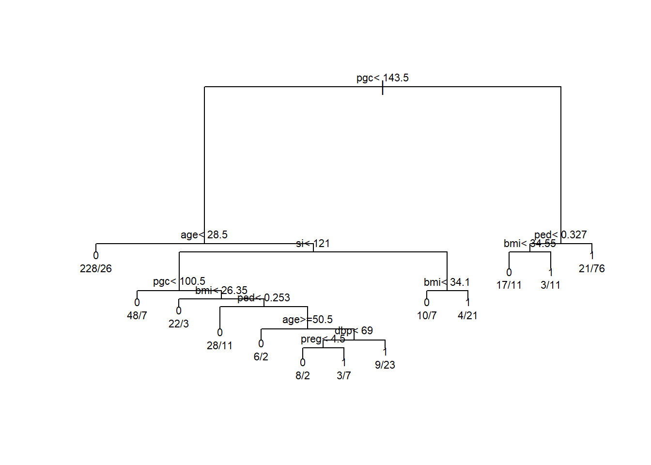
Whether you know it or not, decision trees are an important building block in much of the current machine learning infrastructure. Decision trees are great because they are quite intuitive, easy to explain (even for non-experts), and often have decent predictive performance. Let’s take an example using the Pima Indians Diabetes Database. We can fit a single decision tree predicting the presence of diabetes based on a variety of clinical factors. Without going into too much detail, we will make classification decision rules by implementing binary recursive splitting. For each split in the tree we find the value that maximizes node purity. Following these rules we end up with the tree below:
One of the advantages of this approach is that it is easy to explain to a non-expert. We can see that the first split partitions the sample into two groups: one whose pgc (a measure of blood glucose) is above 143.5 and those who are below. Following the right side of the tree we see that individuals who have a high pgc < 143.5 and a high diabetes pedigree function ped < 0.327 have about a 78% probability of diabetes. From a diagnostic perspective this is really helpful! However, from a strictly performance-based perspective, single decision trees have a few issues:
Limitations:
They tend to have high variance. This means that small changes in the starting state of the data can cause very different trees.
Their performance tends to lag behind other methods. Because a single tree can only explore so much of the predictor space before it begins to overfit, we have to prune these trees back. This means that potentially important interactions farther down the tree path might be unavailable.
Luckily, we have some solutions. One of them is bagging.
Bagging

Bagging (also known as “bootstrap aggregating”) is an approach that works well when you have a single high-variance model. A neat statistical property is that when you average over many high-variance models, the subsequent model will exhibit lower variance overall. We can directly apply this property with our decision trees by creating \(B\) bootstrapped datasets, then fitting \(M\) models to those datasets. Finally, we aggregate the predictions across all the models to create a single ensemble learner. While there are many packages that can handle this efficiently in R, I’m going to code a bit of it from scratch to illustrate how simple (yet powerful) this idea is.
Bagging Functions
Lets start by writing out the code to perform bagging on our decision tree model. To start, we will need to define a few functions: (1) a function to sample the rows from our training dataset with replacement, (2) A function to run an rpart model, given some data and a model formula, and (3) a function to generate predictions on some new data. Step 1 will handle the bootstrap replication, step 2 will handle the model fitting, and step 3 will handle the ensambling into a single prediction.
# (1) Function to sample rows with replacement
boot_data <- function(df){
  return(df[sample(1:nrow(df), replace = T),])
}

# (2) Function to run an Rpart model, provided
# `x` data and a model formula `form`
rpart_fit <- function(x, form){
  rpart(form, data = x, method = "class")
}

# (3) Function to get predictions from models on new data
get_pred <- function(x, newdat) {
  p <- predict(x, newdata = newdat)

  return(p[, 2])
}
Fitting the Bagging Model
Now that we’ve defined the important functions, let’s run through the process. To start, we are going to use a for loop to generate \(B\) boostrapped datasets (here, just using 100 for speed purposes). We’ll then save all these datasets into a list and train a classification tree model on each of them using a vectorized approach (generally preferred over for loops in R). Then we will aggregate predictions over all of the trees to come up with our final ensemble model.
# define number of bootstrap iterations
B = 100

# set up list to hold models, length B
blist <- vector(mode = "list", length = B)

# bootstrap B models
for(i in 1:B)
  blist[[i]] <- boot_data(pima_train)

# run vectorized model, adding our model formula in
bag_fit <- lapply(blist, rpart_fit, form = diabetes ~ .)
We should see that this gives us a list of \(B\) models. If we wanted, we could inspect any individual model by examining the bag_fit object. We’re going to use this list of models to make predictions on our test set, then aggregate those predictions (the ensambling step).
# average over B models
b_avg <- do.call(rbind, (lapply(bag_fit, get_pred, pima_test)))
The b_avg matrix contains 100 rows (one row for each bootstrap iteration) and 154 columns (one column for each observation in the test dataset). Therefore, for every observation we have 100 predictions coming from 100 different models.
dim(b_avg)[1] 100 154It’s handy to have the data in this format because all we have to do now is get the column averages for each observation in the test dataset. Here, we’ll just use the apply function to get the column means.
# get the average over all B models
b_final <- apply(b_avg, 2, mean)
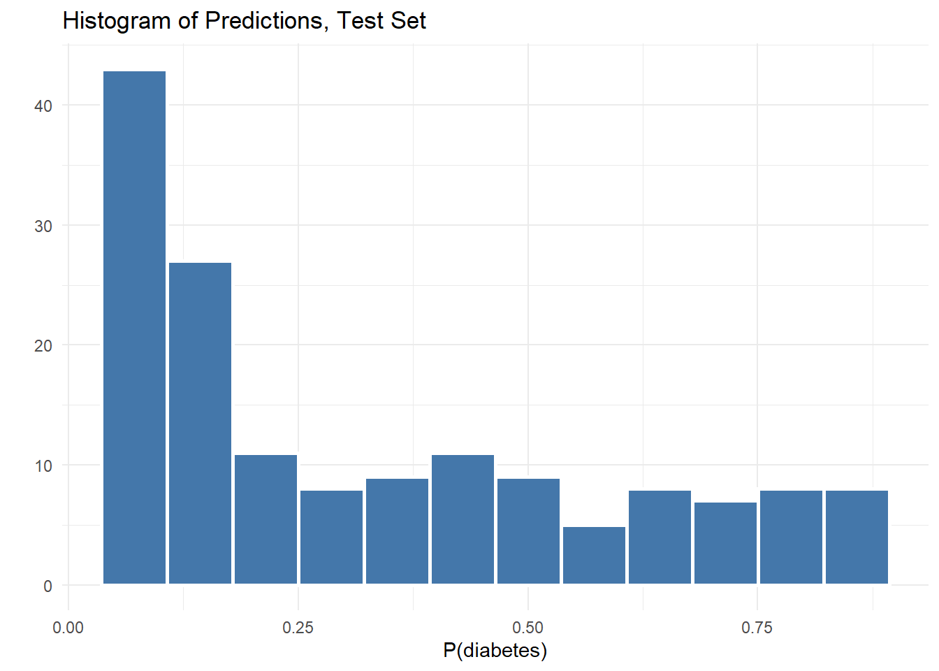
That’s it! Now we have a single vector of predicted values for our test set. We can visualize this quickly with a histogram.

Evaluation: Bagging vs. Decision Tree
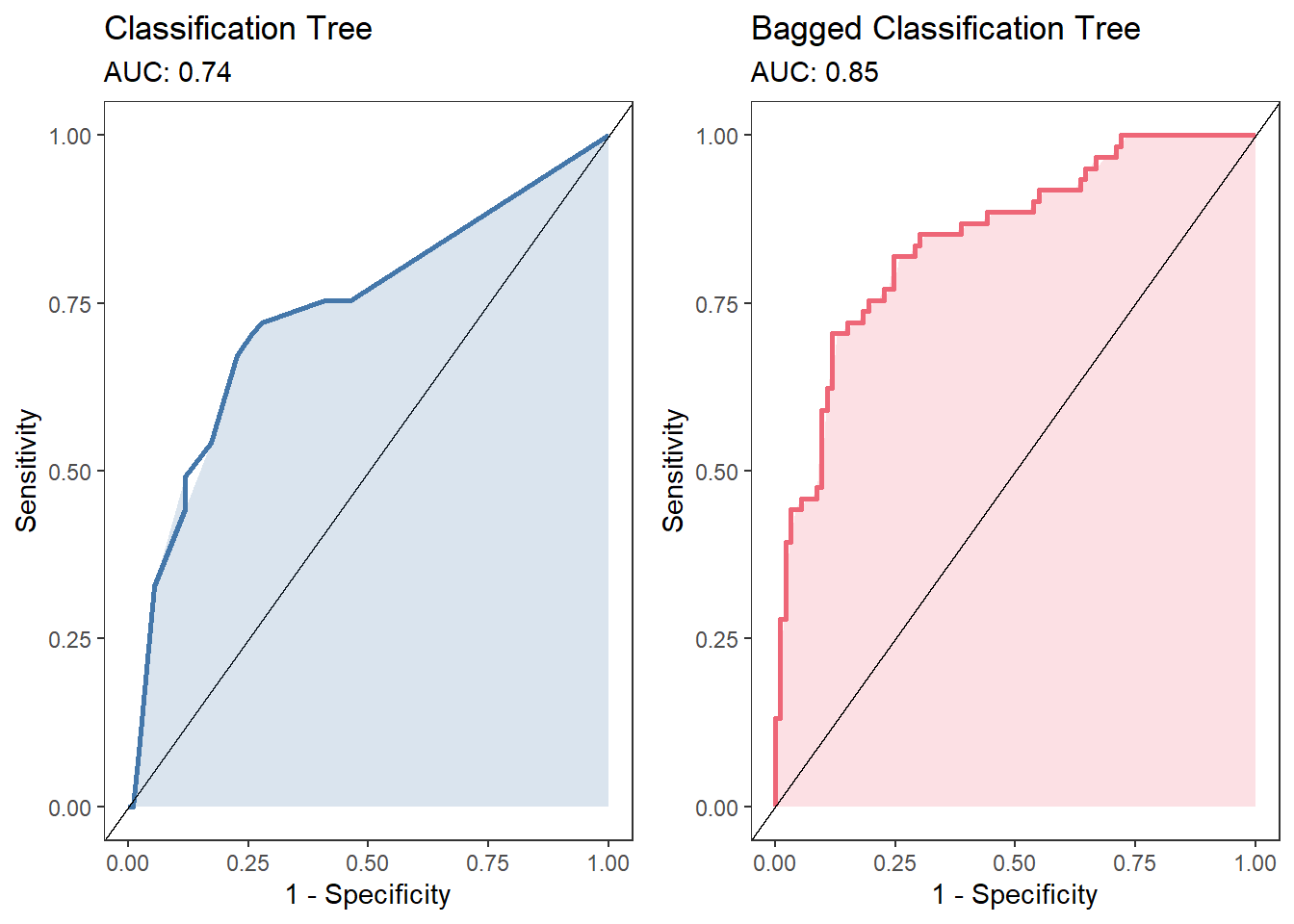
We can test whether the performance of our bagged model is better than the single classification tree. Here, we can calculate the area under the curve (AUC) for both models (we could, just as easily, use any other metric). The plot below shows that there is a fairly substantial increase in AUC from the single model .74 to the bagged model .85.

Random Forests
A notable limitation of bagging is that the models fit to the trees will tend to be highly correlated. This is especially the case if one or two variables have very strong predictive value. Regardless of the bootstrapping step, most trees will choose the same initial splits, which will make many trees that are quite similar. We can de-correlate the trees somewhat by restricting which variables each model is allowed to fit on. This is known as a random forest. This is actually quite similar to the bagging step, except we will choose a proportion of the total number of variables to randomly allocate to each model.
In short, we can augment the bagging step by also randomly selecting a number of parameters for each bagged model. This means that any individual model is only allowed to see a subset of the total number of variables. By default we often use \(\sqrt{p}\) as a starting point for the number of parameters to sample for each tree. Here, that’s roughly \(p = 3\). Below, we’ll create an additional function to sample the dataframe during the bagging step.
# function to randomly select variables
# including outcome variable y
sample_p <- function(df, y, maxp = 3) {
  x <- df[!names(df) %in% y]
  x <- df[sample(names(x), maxp)]

  return(cbind(x, df[y]))
}
Now we can repeat the process for bagging, but just wrap our original boostrapping function inside of the sample_p function, which will implement the step needed for the random forest procedure.
rflist <- vector(mode = "list", length = B)

for(i in 1:B)
  rflist[[i]] <- sample_p(boot_data(pima_train), y = "diabetes")
Now we just follow the same steps from above, swapping in our new rflist.
# fit models
rf_fit <- lapply(rflist, rpart_fit, form = diabetes ~ .)

# get predictions on new data
rf_avg <- do.call(rbind, (lapply(rf_fit, get_pred, pima_test)))

# average over predictions
rf_final <- apply(rf_avg, 2, mean)
Comparing All Three Models
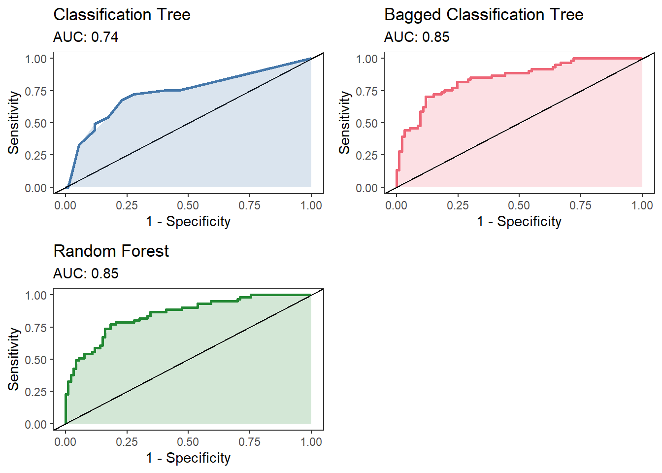
Here we see that bagging results in a fairly substantial improvement over the individual classification tree, but the random forest approach is pretty similar to the bagged model. In all fairness, this is a pretty tiny dataset with only a few important variables. Likely most of the predictive power is coming from just a subset of the total number of variables (primarily pgc, age, and bmi). Regardless we can see that both of these approaches improve over a single model and don’t require much additional coding.

Replication Code
Code to reproduce the analyses here can be found below. The pima dataset can be downloaded here.
Show the code
# load packages
library(tidyverse)
library(rpart)
library(pROC)

# seed for repro
set.seed(5344)

pima <- read_csv("~/pima.csv")

pima_train <- sample_frac(pima, .8)
pima_test <- anti_join(pima, pima_train)

# FUNCTIONS
#-------------------#

# (1) Function to sample rows with replacement
boot_data <- function(df){
  return(df[sample(1:nrow(df), replace = T),])
}

# (2) Function to run an Rpart model, provided
# `x` data and a model formula `form`
rpart_fit <- function(x, form){
  rpart(form, data = x, method = "class")
}

# (3) Function to get predictions from models on new data
get_pred <- function(x, newdat) {
  p <- predict(x, newdata = newdat)

  return(p[, 2])
}

# (4) Function for random forest parameter selection
sample_p <- function(df, y, maxp = 3) {
  x <- df[!names(df) %in% y]
  x <- df[sample(names(x), maxp)]

  return(cbind(x, df[y]))
}

# SINGLE DECISION TREE
#-------------------#
dt_fit <- rpart(diabetes ~ ., data = pima_train, method = "class")

# Plot Results
par(xpd = NA)
plot(dt_fit)
text(dt_fit, use.n = TRUE, cex = .7)

# BAGGING
#-------------------#
# define number of bootstrap iterations
B = 100

# set up list to hold models, length B
blist <- vector(mode = "list", length = B)

# bootstrap B models
for(i in 1:B)
  blist[[i]] <- boot_data(pima_train)

# run vectorized model, adding our model formula in
bag_fit <- lapply(blist, rpart_fit, form = diabetes ~ .)

# get predictions on new data
b_avg <- do.call(rbind, (lapply(bag_fit, get_pred, pima_test)))

# average over predictions
b_final <- apply(b_avg, 2, mean)

# RANDOM FOREST
#---------------------#
rflist <- vector(mode = "list", length = B)

for(i in 1:B)
  rflist[[i]] <- sample_p(boot_data(pima_train), y = "diabetes")

# fit models
rf_fit <- lapply(rflist, rpart_fit, form = diabetes ~ .)

# get predictions on new data
rf_avg <- do.call(rbind, (lapply(rf_fit, get_pred, pima_test)))

# average over predictions
rf_final <- apply(rf_avg, 2, mean)


# EVALUATION
#---------------------#

# Use pROC for AUC

# single tree
roc(pima_test$diabetes, get_pred(dt_fit, newdat = pima_test))

# bagging and random forest
roc(pima_test$diabetes, b_final)
roc(pima_test$diabetes, rf_final)