Model
The model for the analysis will be a simple dynamic AR(1) panel. Its specification can be written, following (Bond 2002), as:
\[\begin{equation} y_{it} = \alpha y_{it-1} + \eta_i + v_{it} \end{equation}\]
with the process being stationary (\(|\alpha|<1\)). We consider the following set of assumptions regarding the individual effect \(\eta_i\) and the innovation \(v_{it}\):
- zero mean
- homoskedasticity
- no serial autocorrelation of the innovation
- no correlation between the individual effect and the innovation
\[\begin{equation} \mathbb{E}[v_{it}] = \mathbb{E}[\eta_i] = 0 \end{equation}\]
\[\begin{equation} \mathbb{E}[v_{it}^2] = \sigma^2_v ; \mathbb{E}[\eta_i^2] = \sigma^2_{\eta} \end{equation}\]
\[\begin{equation} \mathbb{E}[v_{it}v_{is}] = 0 \ \ \ \forall s \neq t \end{equation}\]
\[\begin{equation} \mathbb{E}[\eta_iv_{it}] = 0 \end{equation}\]
Data
We will work with the dataset RDPerfComp, present in the pder package (Croissant and Millo 2008), consisting of employment data of US manufacturing companies. The original dataset can be found in (Blundell and Bond 2000).
The balanced panel contains yearly observations of the log employment of 509 firms (\(N = 509\)) from 1982 to 1989 (\(T = 8\)), so it can be classified as a ‘large \(N\), small \(T\)’ panel.
The data is shown in an interactive table (Table 1) and summarized graphically (Figure 1)
Table 1. Panel of US firms
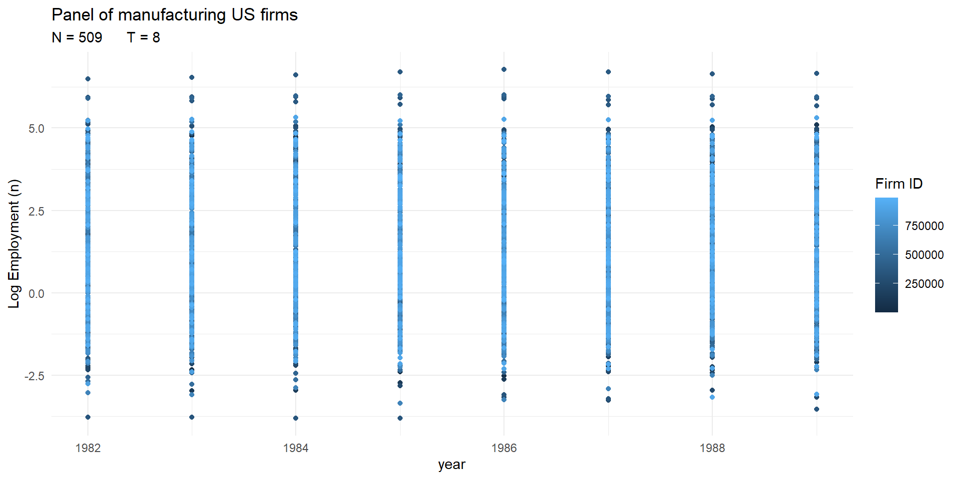
Figure 1. Panel of US firms
The dependent variable \(y_{it}\) represents log employment. In the subsequent code,n is represented by \(y_{it}\),lag(n,p) is the expression for series in lags \(y_{it-p}\), and diff(n) denotes the series in first differences \(\Delta y_{it}\).
Estimation
Several estimation methods for micro panels are considered and implemented through the use of the functions plm and pgmm (Croissant and Millo 2008). These methods are:
- OLS
- Within
- Anderson-Hsiao (2SLS)
- Difference GMM (1-step and 2-steps)
panel_OLS <- plm('n ~ lag(n) - 1',
                 panel_wage,
                 model = 'pooling')

panel_within <- plm('n ~ lag(n) - 1',
                    panel_wage,
                    model = 'within')

panel_ahsiao <- plm('diff(n) ~ lag(diff(n),1) - 1 | lag(n, 2)',
                    panel_wage,
                    model = 'pooling')

panel_one_step_gmm <- pgmm(n ~ lag(n,1) - 1 | lag(n, 2:99),
                    panel_wage,
                    transformation = 'd',
                    model = 'onestep',
                    effect = 'individual')

panel_two_steps_gmm <- pgmm(n ~ lag(n,1) - 1 | lag(n, 2:99),
                    panel_wage,
                    transformation = 'd',
                    model = 'twosteps',
                    effect = 'individual')
Additionally, other computations and tests are calculated:
- Robust (Windmeijer) standard errors for the estimators, computed with
vcovHC
sd_robust_ols <- sqrt(vcovHC(panel_OLS)[1])
sd_robust_within <- sqrt(vcovHC(panel_within)[1])
sd_robust_one_step <- sqrt(vcovHC(panel_one_step_gmm)[1])
sd_robust_two_steps <- sqrt(vcovHC(panel_two_steps_gmm)[1])- Arellano-Bond test for serial correlation of the innovations, using
mtest
m1_one_step <- mtest(panel_one_step_gmm, order = 1)
m2_one_step <- mtest(panel_one_step_gmm, order = 2)

m1_two_steps <- mtest(panel_two_steps_gmm, order = 1)
m2_two_steps <- mtest(panel_two_steps_gmm, order = 2)- Sargan-Hansen test of overidentifying restrictions, computed with the function
sargan
Results
| OLS | Within | Anderson-Hsiao | One step Difference-GMM | Two steps Difference-GMM | |
|---|---|---|---|---|---|
| AR(1) coefficient estimate | 0.9959 | 0.7219 | 0.8006 | 0.8634 | 0.8648 |
| Standard Error | 0.0014 | 0.0123 | 0.1071 | 0.0138 | 0.0597 |
| Robust Standard Error | 0.0014 | 0.0213 | 0.0670 | 0.0820 | |
| Arellano-Bond test p-value (lag 1) | 0.0000 | 0.0000 | |||
| Arellano-Bond test p-value (lag 2) | 0.8433 | 0.8451 | |||
| Sargan-Hansen test | 0.0014 | 0.0014 |
As expected, the OLS estimate shows a high value as the OLS estimator is biased upwards (\(plim \ \hat{\alpha}_{OLS} > \alpha\)). Conversely, the within estimate takes a low value, being its estimator biased downwards (\(plim \ \hat{\alpha}_{Within} < \alpha\)). In the case of the GMM estimators, the hypothesis of no serial correlation of \(v_{it}\) (in levels) is not rejected, although the validity of instruments is rejected by the Sargan-Hansen test.
References
Blundell, Richard, and Stephen Bond. 2000. “GMM Estimation with Persistent Panel Data: An Application to Production Functions.” Econometric Reviews 19 (3): 321–40. https://doi.org/10.1080/07474930008800475.
Bond, Stephen R. 2002. “Dynamic Panel Data Models: A Guide to Micro Data Methods and Practice.” Portuguese Economic Journal 1 (2): 141–62. https://EconPapers.repec.org/RePEc:spr:portec:v:1:y:2002:i:2:d:10.1007_s10258-002-0009-9.
Croissant, Yves, and Giovanni Millo. 2008. “Panel Data Econometrics in R: The plm Package.” Journal of Statistical Software 27 (2): 1–43. https://doi.org/10.18637/jss.v027.i02.
Guillermo Corredor (2021), guillermo.corredor.log@gmail.com↩︎