R @ Ewha 2020
2020-09-24
1 Week1: Introduction to R
1.1 Reading for this lecture
1.2 Two ways to read lecture notes
- On the shinyapps server
- You can access lecture notes on the web through the link provided in cyber campus
- On you local computer
- You can compile
week1_introduction_to_R.Rmdfile in RStudio.
- I will post how to compile
week1_introduction_to_R.Rmdfile in our cyber campus.
- You can compile
1.3 Welcome
Hi everyone, welcome to the course :) This is the introduction to R course at Ewha Womans University in 2020.
R is a great programming language for statistical analysis and data science. I hope you enjoy R in this course and find many useful applications for your own field.
This course is designed for those who don’t have any programming background, especially in social science major.
Today, I will just introduce R, RStudio, and some basic terminologies
In this lecture note,
this fontrepresents R keyword/packages and this font represents hyperlink you can click.
1.4 Why R?
- R is a language designed for statistical analysis.
- R is very popular especially in academia. Many researchers first implement their experimental methods in statistics and machine learning using R. So you can use many cutting-edge algorithms in R by downloading many packages in R.
- R provides many tools for publication-quality data visualization.
- Data visualization help you to understand your data and present your findings to others. In this lecture, you will learn
ggplot2package for data visualization.
- Data visualization help you to understand your data and present your findings to others. In this lecture, you will learn
- R provides many tools for data wrangling.
- You need to transform your own data into a useful form for visualization and modeling. This process is often called data wrangling. In this lecture, you will learn many packages in
tidyverse(e.g.,dplyr,tidyr,purrr,stringr) for data wrangling.
- Data wrangling is an important skill in these days to effectively handle data from diverse sources (e.g., facebook, twitter, fMRI, eyetracker, EEG). For example, many servers store user data in the JSON format for data exchange, and so you need to handle JSON files if you want to use user data for your analysis.
- You need to transform your own data into a useful form for visualization and modeling. This process is often called data wrangling. In this lecture, you will learn many packages in
- R has active and supportive communities.
- You can find many useful resources from those communities. For example, the
bookdownis an R package for writing books, and bookdown.org provides useful R books written with thebookdownpackage for free. In the bookdown.org, you will find our textbook for this class, which is R for Data Science.
- You can find many useful resources from those communities. For example, the
- R is a free open source software.
1.5 R vs Python
Python is another great programming language. You can find many interesting debates over R vs Python on the internet. Here is an example.
In short, Python is a general-purpose programming language used for a wide variety of applications (e.g., data science, web development, database), whereas R is a programming language focusing on data science.
One of the goals of this course is to give you an opportunity for exploring R so that you can make a decision about which language is best for your purpose. You may need both languages :)
“Generally, there are a lot of people who talk about R versus Python like it’s a war that either R or Python is going to win. I think that is not helpful because it is not actually a battle. These things exist independently and are both awesome in different ways.”
— Hadley Wickham
1.6 Let’s install R to your local computer
Please install base R for your own operating system from https://cloud.r-project.org/
You will find lots of videos demonstrating installing process on YouTube.
1.7 Let’s install RStudio to your local computer
Please install FREE version of RStudio for your own operating system from https://rstudio.com/products/rstudio/download/.
RStudio is an integrated development environment (IDE) for R.
- R will do all the calculations for you.
- RStudio is just an convenient interface between you and R.
- So, you can just launch RStudio to use R.
You will find lots of videos demonstrating installing process on YouTube.
1.8 Three ways you can use R in this course
- You can use RStudio in your local computer.
- You can launch RStudio you downloaded above from your Windows or Mac computers.
- You can use RStudio Cloud for free.
- RStudio Cloud allows you to use RStudio in the Web browser.
- You can get free account in RStudio Cloud here.
- RStudio Cloud allows you to use RStudio in the Web browser.
- You can use the interactive code chunk in this lecture note.
The interactive code chunk in this lecture note was created using learnr package
If you see Do It! throughout this semester, it means that I want you to actually do something :) The Do It! below contains the interactive code chunk. You can actually run R commands in this interactive code chunk and see the results instantly.
- Do It (1-1)
- Please type the following R commands in the interactive code chunk and click
Run Codebutton on the right side to see what happen:ggplot(data = diamonds, aes(x = carat, y = price, color = color)) + geom_point(). This code uses theggplot2package, an R package for data visualization. You will learn theggplot2package next week. For now, just type the code in the interactive code chunk.
- Please type the following R commands in the interactive code chunk and click
1.9 Useful R resources
You can find many useful resources (many of them are FREE) for learning R on the internet.
Free ebooks
bookdown is an R package that helps you to write and publish books using RStudio. Please check wonderful books on the site. You can freely read those books online.
In this site, you can find our textbook, R for Data Science (Hadley Wickham).
If you are interested in writing and publishing books on the internet like the ones on the bookdown website, please read bookdown: Authoring Books and Technical Documents with R Markdown (Yihui Xie). (This class will not cover this topic)
As you may already know, many researchers around the world create R packages and share with others through R package systems. If you are interested in creating your own R package, please read R Packages (Hadley Wickham). (This class will not cover this topic)
If you think you want to learn more advanced R at the end of this course, please read Advanced R (Hadley Wickham). (This class will not cover this topic)
If you prefer to read those books in Korean, try to translate books using the Chrome web browser: open the ebooks using Chrome web browser, click right mouse button, and choose “translate in Korean.”
You may already notice that the name “Hadley Wickham” appears here and there. Hadley Wickham contributes a lot to R community as a chief scientist at RStudio, creator of
tidyversepackage (ggplot2,dplyr,tidyr,stringr, etc.), and authors of many books. You can find more about Hadley in Hadley’s website.
RStudio Cheatsheets
One of the strengths of R is its package system. There are more than 16,000 packages that extend the functionality of base R. However, it’s difficult to remember all the details of such large number of packages.
RStudio provides RStudio Cheatsheets which summarize features of some important R packages in one or two pages. The cheatsheets will be nice references when you actually work with R for your own project.
1.10 R Packages
R packages are the collections of functions and data sets developed by the R community. Currently, the Comprehensive R Archive Network(CRAN) repository contains more than 16,000 packages. A list of R packages are available here. Packages increase the power of R by improving and extending base R.
Installing vs Loading
- Installing means you download the package files from the CRAN repository to your local computer. You only need to install a package once. An R function named
install.packages()is used to install packages. - Loading means you load functions and data in the package onto your computer memory. Loading functions and data of all packages to memory is inefficient in terms of computers’ memory management. So you only load a package onto memory when you need it. In other word, whenever you want to use functions in a package, you need to load the package that contains the functions. An R function named
library()is used to load packages. - For example, we will learn the
ggplot2package for data visualization from week 2. In order to use functions inggplot2, you need to install theggplot2package by runninginstall.packages("ggplot")once, and load the package by runninglibrary(ggplot2)whenever you need the package.
- Installing means you download the package files from the CRAN repository to your local computer. You only need to install a package once. An R function named
1.11 Base R vs Tidyverse
- Base R
- Base R refers to the collection of functions and packages that come with a clean install of R.
- Many packages extend Base R.
- You will learn Base R later in this class.
- Here’s a cheatsheet for Base R
- Tidyverse
- The
tidyversepackage is a collection of packages for more efficient data science in R. - In the
tidyversepackage, thedplyr,tidyr,ggplot2, andpurrrpackages provide many useful functions for efficient data transformation, data tidying, data visualization, and iteration, respectively. - Our textbook R for Data Science (Hadley Wickham) is all about tidyverse.
- A significant portion of this class will be devoted to learning various packages in tidyverse.
- You can quickly check the features of core tidyverse packages here.
- The
1.12 R script file vs R markdown file
Both R script and markdown files are just a plain text file, meaning that you can open and edit with Windows’ notepad or any other text editor.
In an R script, you can only include R codes (with comments), whereas in an R markdown, you can include interactive code chunk and your text. In this class, we will mainly use and practice R markdown.
1.13 R markdown
Along with tidyverse, R markdown is one of my favorite part in R.
R markdown is a file format that can be converted into many different documents such as HTML, PDF, Microsoft Word, and other dynamic documents. That is, it’s a nice example of one source multi use.
For example, this R markdown text file can be converted into this nice HTML.
This lecture notes were also made with R markdown :)
Let’s watch a short introductory video for R markdown.
You will be amazed how many nice documents can be created from a simple R markdown text file. Please check nice documents from R markdown here.
These days, how you present your work is just as important as what you present. If you learn R markdown, you can present your contents in many different wonderful formats.
Here’s R markdown cheatsheet.
If you are serious in R markdown, please read R Markdown: The Definitive Guide(Yihui Xie, J. J. Allaire, Garrett Grolemund).
In this class, we will cover the basic of R markdown.
Let’s explore R markdown. You can open a new R markdown template by going
File > New File > R Markdown...
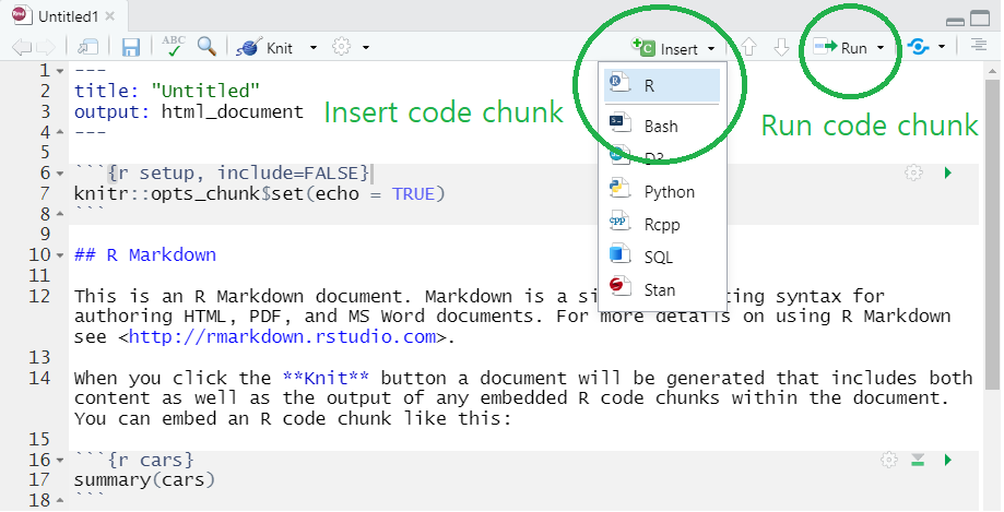
R Markdown template in RStudio
- Notice that R markdown contains white and gray areas. The white area is where your text goes, whereas the gray area is where your R code goes.
- You can create a code chunk by
- clicking
insertand chooseRon the menu (check the green circle on the above image) or - typing a short cut key or
- Windows:
Ctrl + Alt + I - Mac:
Cmd + Option + I
- Windows:
- clicking
- You can run the code in a code chunk by
- clicking
Runon the menu (check the green circle on the above image) or - typing
Ctrl + Enterwhen you place your cursor at the line of the code you want to run
- clicking
- You can find more information on code chunks here
- You can create a code chunk by
- Again, the biggest benefit of using R markdown is that you can create multiple output formats (e.g.s, HTML, PDF, MS Word, Beamer slide, shiny applications, websites).
- For example, you can easily create HTML, PDF, MS Word from your R markdown document by simply clicking
knitbutton and choose the format you want (check the green circle on the below image). - To knit to PDF, you need a Tex typesetting system.
- For example, you can easily create HTML, PDF, MS Word from your R markdown document by simply clicking
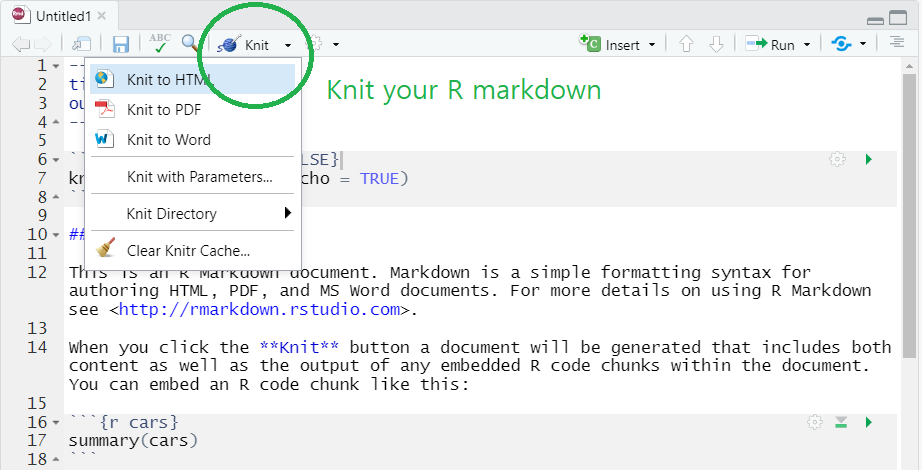
R Markdown template in RStudio
- You can even publish your R markdown to web very easily. I will talk about this another class.
1.14 Let’s get familiar with RStudio
You may not be familiar with RStudio menus and buttons when you launch RStudio for the first time. However, you will get familiar with RStudio very soon.
Let’s watch a short introductory video for RStudio here
Notice that RStudio consists of four panels (or panes)
- Source editor pane
- This is where you can edit your code in R script or R markdown files
- Console pane
- This is where you can execute your code instantly
- Environment pane
- This is where you can see the objects (or variables)
- File/Plots/Packages/Helps pane
- This is where you can see files, plots, packages, and help documents.
- Source editor pane
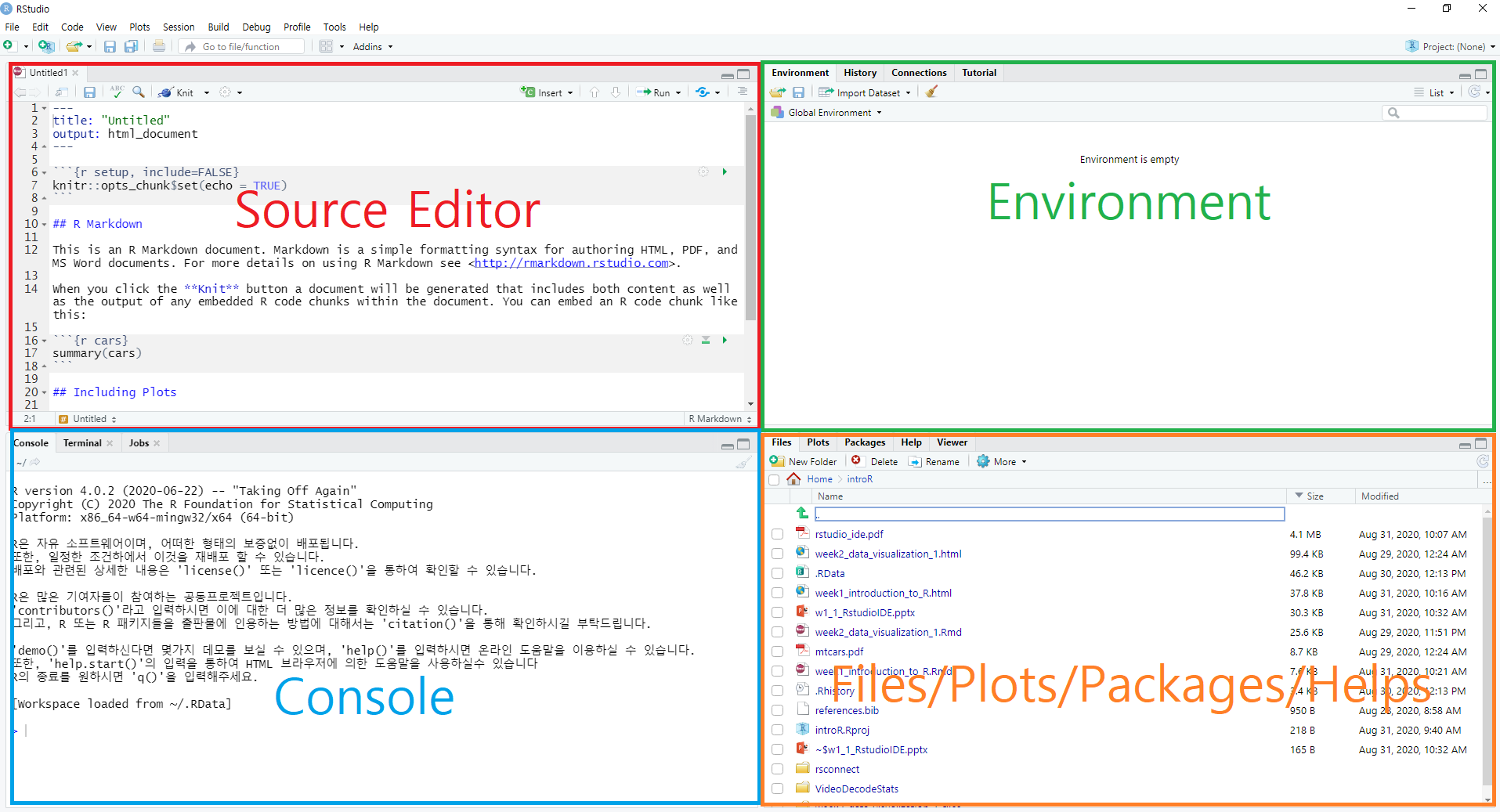
Four main panes in RStudio IDE
- You can find more RStudio features here.
1.15 Things that you can do with R and RStudio
In Ch1 of R for Data Science, the author illustrates the process in typical data science project as follows
- import: read data into R
- tidy, transform: get the original data into our desired form
- visualize: create plots to understand data or to present findings
- model: detect patterns from data
- communicate: tell your findings to others
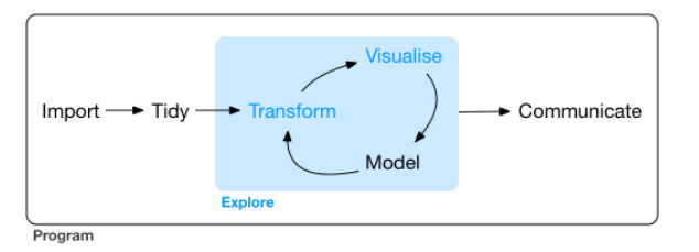
The process in typical data science project
- Let’s go over this process with a simple example using a built-in
mtcarsdata.- For now, just go over each step even though you don’t understand functions used in the code. The only goal of this example is to get you familiar with R and RStudio.
mtcarsis a built-in data in R. The data come from 1974 Motor Trend US magazine, and include fuel consumption and 10 other features of 32 automobiles. You can typemtcarsin your RStudio console to see the data, and type?mtcarsto see the help document for the data.
##                      mpg cyl  disp  hp drat    wt  qsec vs am gear carb
## Mazda RX4           21.0   6 160.0 110 3.90 2.620 16.46  0  1    4    4
## Mazda RX4 Wag       21.0   6 160.0 110 3.90 2.875 17.02  0  1    4    4
## Datsun 710          22.8   4 108.0  93 3.85 2.320 18.61  1  1    4    1
## Hornet 4 Drive      21.4   6 258.0 110 3.08 3.215 19.44  1  0    3    1
## Hornet Sportabout   18.7   8 360.0 175 3.15 3.440 17.02  0  0    3    2
## Valiant             18.1   6 225.0 105 2.76 3.460 20.22  1  0    3    1
## Duster 360          14.3   8 360.0 245 3.21 3.570 15.84  0  0    3    4
## Merc 240D           24.4   4 146.7  62 3.69 3.190 20.00  1  0    4    2
## Merc 230            22.8   4 140.8  95 3.92 3.150 22.90  1  0    4    2
## Merc 280            19.2   6 167.6 123 3.92 3.440 18.30  1  0    4    4
## Merc 280C           17.8   6 167.6 123 3.92 3.440 18.90  1  0    4    4
## Merc 450SE          16.4   8 275.8 180 3.07 4.070 17.40  0  0    3    3
## Merc 450SL          17.3   8 275.8 180 3.07 3.730 17.60  0  0    3    3
## Merc 450SLC         15.2   8 275.8 180 3.07 3.780 18.00  0  0    3    3
## Cadillac Fleetwood  10.4   8 472.0 205 2.93 5.250 17.98  0  0    3    4
## Lincoln Continental 10.4   8 460.0 215 3.00 5.424 17.82  0  0    3    4
## Chrysler Imperial   14.7   8 440.0 230 3.23 5.345 17.42  0  0    3    4
## Fiat 128            32.4   4  78.7  66 4.08 2.200 19.47  1  1    4    1
## Honda Civic         30.4   4  75.7  52 4.93 1.615 18.52  1  1    4    2
## Toyota Corolla      33.9   4  71.1  65 4.22 1.835 19.90  1  1    4    1
## Toyota Corona       21.5   4 120.1  97 3.70 2.465 20.01  1  0    3    1
## Dodge Challenger    15.5   8 318.0 150 2.76 3.520 16.87  0  0    3    2
## AMC Javelin         15.2   8 304.0 150 3.15 3.435 17.30  0  0    3    2
## Camaro Z28          13.3   8 350.0 245 3.73 3.840 15.41  0  0    3    4
## Pontiac Firebird    19.2   8 400.0 175 3.08 3.845 17.05  0  0    3    2
## Fiat X1-9           27.3   4  79.0  66 4.08 1.935 18.90  1  1    4    1
## Porsche 914-2       26.0   4 120.3  91 4.43 2.140 16.70  0  1    5    2
## Lotus Europa        30.4   4  95.1 113 3.77 1.513 16.90  1  1    5    2
## Ford Pantera L      15.8   8 351.0 264 4.22 3.170 14.50  0  1    5    4
## Ferrari Dino        19.7   6 145.0 175 3.62 2.770 15.50  0  1    5    6
## Maserati Bora       15.0   8 301.0 335 3.54 3.570 14.60  0  1    5    8
## Volvo 142E 21.4 4 121.0 109 4.11 2.780 18.60 1 1 4 2- Do It (1-2)
- In the interactive code chunk below, type
mtcarsand clickRun Codeto see the data, and type?mtcarsand clickRun Codeto see the help document for the data.
- In the interactive code chunk below, type
- (transform) If you see the help document of
mtcars, you will seecylis the number of cylinders of the cars. Suppose that we are only interested in the cars with 4 and 6 cylinders. You can first check the frequency of the number of cylinders and then filter the cars with 4 and 6 cylinders as follows:
# Check the frequency of the number of cylinders
# count() is used to get the distribution of values
# count() is a function in `dplyr` package
# So in order to use the count(), you should install and run `dplyr` package first.
# installing dplyr package: install.packages("dplyr")
# loading dplyr package: library(dplyr)
# library(tidyverse) will load core packages in the tidyverse including dplyr
library(tidyverse)
## -- Attaching packages ----------------------------------------------------------- tidyverse 1.3.0 --## √ ggplot2 3.3.2 √ purrr 0.3.4
## √ tibble 3.0.1 √ dplyr 1.0.0
## √ tidyr 1.1.0 √ stringr 1.4.0
## √ readr 1.3.1 √ forcats 0.5.0## -- Conflicts -------------------------------------------------------------- tidyverse_conflicts() --
## x dplyr::filter() masks stats::filter()
## x dplyr::lag() masks stats::lag()## cyl n
## 1 4 11
## 2 6 7
## 3 8 14- Do It (1-3)
- Type
mtcars %>% count(cyl)
- Type
# filter() subsets (or selects) observations
# filter() is also a function in `dplyr` package
# %>% is called a `pipe`, can you guess the meaning?
# function A %>% function B:
# the pipe delivers the outcome of a function A as an input of funciton B
# %>% is a feature of `magrittr` package. We will talk this later.
mtcars %>%
  filter(cyl %in% c(4,6)) %>%
  count(cyl)
## cyl n
## 1 4 11
## 2 6 7- Do It (1-4)
- Type
mtcars %>% filter(cyl %in% c(4,6)) %>% count(cyl)
- Type
- (visualize) We transformed our data
mtcarsinto our desired form, and now we want to visualize our relationship of interest. Suppose that we are interested in the relationship betweenmpg(miles per gallon or kilometers per liter in Korean) anddisp(engine size). We can create a scatter plot betweenmpganddispfor our visual inspection of the relationship using theggplot2package.
# you will learn `ggplot2` package next week.
# for not, it's ok to just know ggplot2 is a package in tidyverse for data visualization
mtcars %>%
  filter(cyl %in% c(4,6)) %>%
ggplot(aes(x = disp, y = mpg)) + geom_point() 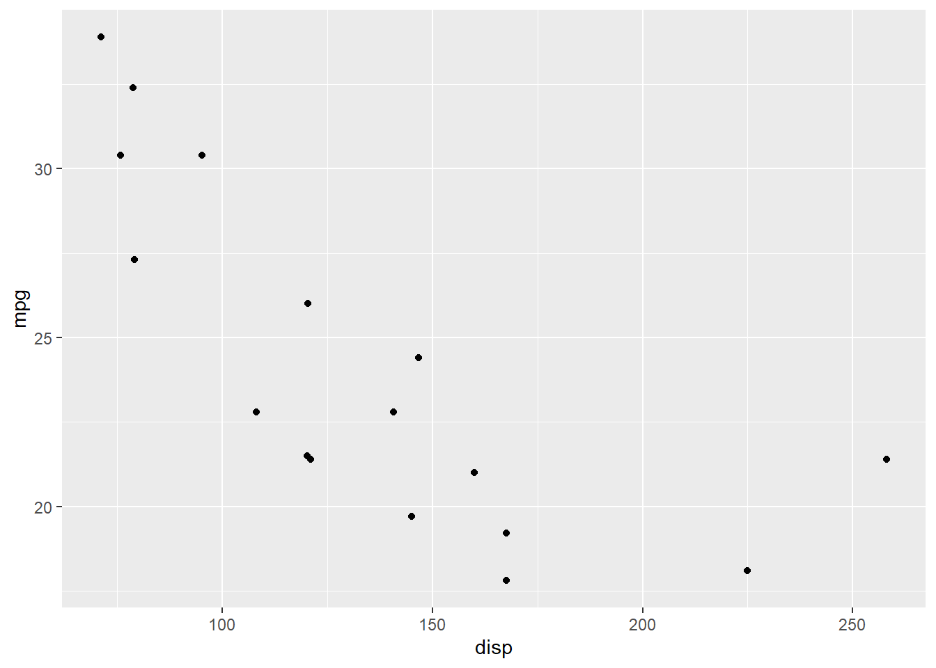
# you can even fit a line to the data and plot it by adding `geom_smooth()`
mtcars %>%
  filter(cyl %in% c(4,6)) %>%
  ggplot(aes(x = disp, y = mpg)) + geom_point() + geom_smooth(method = "lm")
## `geom_smooth()` using formula 'y ~ x'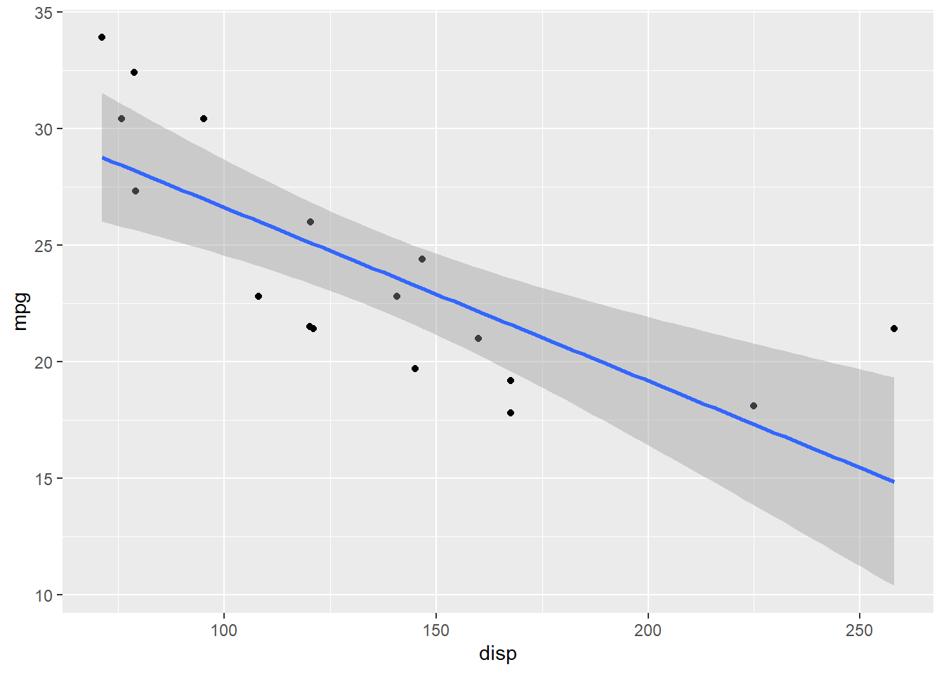
- (model) We visualized our relationship of interest, and now we want to model the relationship with a line. The code below run a simple regression to the filtered data (i.e., cars with only 4 and 6 cylinders), and report regression coefficients.
# lm() is a function in Base R to fit linear models (or simply regression)

mtcars2 <- mtcars %>%
  filter(cyl %in% c(4,6))

summary(lm(mpg ~ disp, data = mtcars2))
##
## Call:
## lm(formula = mpg ~ disp, data = mtcars2)
##
## Residuals:
## Min 1Q Median 3Q Max
## -3.7873 -3.0124 -0.8294 1.7969 6.5373
##
## Coefficients:
## Estimate Std. Error t value Pr(>|t|)
## (Intercept) 34.05456 2.30665 14.764 9.69e-11 ***
## disp -0.07439 0.01599 -4.651 0.000266 ***
## ---
## Signif. codes: 0 '***' 0.001 '**' 0.01 '*' 0.05 '.' 0.1 ' ' 1
##
## Residual standard error: 3.345 on 16 degrees of freedom
## Multiple R-squared: 0.5748, Adjusted R-squared: 0.5483
## F-statistic: 21.63 on 1 and 16 DF, p-value: 0.0002663- Do It (1-5)
- Run above regression in the interactive code chunk below
1.16 Homework (this HW will not be graded !!)
- Do the following:
- create an R markdown template by going
File > New File > R Markdown...and - replicate Do It (1-2), Do It (1-3), Do It (1-4), and Do It (1-5) (You need to create a code chunk. Check
1.12 R Markdownsection to create a code chunk) - create an HTML, PDF, and MS word documents by kniting the R markdown (Check
1.12 R Markdownto knit your R markdown)
- note that you need Tex system for PDF
- You can add your own text in white space for your own report.
- Next week, I will post a video demonstrating how I did for this HW :)
- create an R markdown template by going
1.17 Comments of Week1 lecture
The goal of week 1 lecture is just to introduce basic concepts and terminology in R and RStudio, and to get you familiar with RStudio interface. The only way you can improve your programming skill is actually write codes. Please play with RStudio as much as you can, and practice the code in the lecture material.
Next week, we will talk about our first tidyverse package
ggplot2for data visualization. From next week, I will provide you more videos demonstrating how actually run codes in RStudio.To give you enough time to get familiar with R materials and lecture formats, we will not have any quiz until week 3.
Please feel free to post any question regarding course materials on the cyber campus.