Multiple Regression

Introduction

In Chapter 1 there is only one explanatory variable. However, in many questions we expect multiple explanations. In determining a person’s income, the education level is very important. There is clear evidence that other factors are also important, including experience, gender and race. Do we need to account for these factors in determining the effect of education on income?

Yes. In general, we do. Goldberger (1991) characterizes the problem as one of running a short regression when the data is properly explained by a long regression. This chapter discusses when we should and should not run a long regression.
It also discusses an alternative approach. Imagine a policy that can affect the outcome either directly or indirectly through another variable. Can we estimate both the direct effect and the indirect effect? The chapter combines OLS with directed acyclic graphs (DAGs) to determine how a policy variable affects the outcome. It then illustrates the approach using actual data on mortgage lending to determine whether bankers are racist or greedy.

Long and Short Regression

Goldberger (1991) characterized the problem of omitting explanatory variables as the choice between long and short regression. The section considers the relative accuracy of long regression in two cases: when the explanatory variables are independent of each other, and when the explanatory variables are correlated.

Using Short Regression

Consider an example where true effect is given by the following long regression. The dependent variable $y$ is determined by both $x$ and $w$ (and $\upsilon$).

$$\begin{array}{}\text{(1)}& y_i=a+b{x}_i+c{w}_i+{\upsilon }_i\end{array}$$

In our running example, think of $y_i$ as representing the income of individual $i$. Their income is determined by their years of schooling ($x_i$) and by their experience ($w_i$). It is also determined by unobserved characteristics of the individual (${\upsilon }_i$). The last may include characteristics of where they live such as the current unemployment rate.

We are interested in estimating $b$. We are interested in estimating returns to schooling. In Chapter 1, we did this by estimating the following short regression.

$$\begin{array}{}\text{(2)}& y_i=a+b{x}_i+{\upsilon }_{wi}\end{array}$$

By doing this we have a different “unobserved characteristic.” The unobserved characteristic, ${\upsilon }_{wi}$ combines both the effects of the unobserved characteristics from the long regression (${\upsilon }_i$) and the potentially observed characteristic ($w_i$). We know that experience affects income, but in Chapter 1 we ignore the possibility.

Does it matter? Does it matter if we just leave out important explanatory variables? Yes. And No. Maybe. It depends. What was the question?

Independent Explanatory Variables

Figure 1: Two variable causal graph.

Figure 1 presents the independence case. There are two variables that determine the value of $Y$, these are $X$ and $W$. If $Y$ is income, then $X$ may be schooling while $W$ is experience. However, the two effects are independent of each other. In the figure, independence is represented by the fact that there is no line joining $X$ to $W$, except through $Y$.

Consider the simulation below and the results of the various regressions presented in Table 1. Models (1) and (2) show that it makes little difference if we run the short or long regression. Neither of the estimates is that close, but that is mostly due to the small sample size. It does impact the estimate of the constant; can you guess why?

Dependent Explanatory Variables

Figure 2: Two variable causal graph with dependence.

Short regressions are much less trustworthy when there is some sort of dependence between the two variables. Figure 2 shows the causal relationship when $X$ and $W$ are related to each other. In this case, a short regression will give a biased estimate of $b$ because it will incorporate $c$. It will incorporate the effect of $W$. Pearl and Mackenzie (2018) calls this a backdoor relationship because you can trace a relationship from $X$ to $Y$ through the backdoor of $U$ and $W$.

Models (3) and (4) of Table 1 present the short and long estimators for the case where there is dependence. In this case we see a big difference between the two estimators. The long regression gives estimates of $b$ and $c$ that are quite close to the true values. The short regression estimate of $b$ is considerably larger than the true value. In fact, you notice the backdoor relationship. The estimate of $b$ is close to 7 which is the combined value of $b$ and $c$.

Simulation with Multiple Explanatory Variables

The first simulation assumes that $x$ and $w$ affect $y$ independently. That is, while $x$ and $w$ both affect $y$, they do not affect each other nor is there a common factor affecting them. In the simulations, the common factor is determined by the weight $\alpha$. In this case, there is zero weight placed on the common factor potentially affecting both observed characteristics.

set.seed(123456789)
N <- 1000
a <- 2
b <- 3
c <- 4
u_x <- rnorm(N)
alpha <- 0
x <- x1 <- (1 - alpha)*runif(N) + alpha*u_x
w <- w1 <- (1 - alpha)*runif(N) + alpha*u_x
u <- rnorm(N)
y <- a + b*x + c*w + u
lm1 <- lm(y ~ x)
lm2 <- lm(y ~ x + w)

The second simulation allows for dependence between $x$ and $w$. In the simulation this is captured by a positive value for the weight that each characteristic places on the common factor $u_x$. Table 1 shows that in this case it makes a big difference if a short or long regression is run. The short regression gives a biased estimate because it is accounting for the effect of $w$ on $y$. Once this is accounted for in the long regression, the estimates are pretty close to the true value.

alpha <- 0.5
x <- x2 <- (1 - alpha)*runif(N) + alpha*u_x
w <- w2 <- (1 - alpha)*runif(N) + alpha*u_x
y <- a + b*x + c*w + u
lm3 <- lm(y ~ x)
lm4 <- lm(y ~ x + w)

The last simulation suggests that we need to take care not to overly rely on long regressions. If $x$ and $w$ are highly correlated, then the short regression gives the dual effect, while the long regression presents garbage.¹

alpha <- 0.95
x <- x3 <- (1 - alpha)*runif(N) + alpha*u_x
w <- w3 <- (1 - alpha)*runif(N) + alpha*u_x
y <- a + b*x + c*w + u
lm5 <- lm(y ~ x)
lm6 <- lm(y ~ x + w)

Table 1: OLS estimates of short and long regressions. Models (1) and (2) compare short and long regressions when there is no dependence between $x$ and $w$. Models (3) and (4) present the same comparison with dependence. Models (5) and (6) are for the strong dependence case. In order, from top to bottom, the true values are 3, 4 and 2.

	(1)	(2)	(3)	(4)	(5)	(6)
(Intercept)	3.983	2.149	2.142	2.071	2.075	2.077
	(0.099)	(0.082)	(0.046)	(0.036)	(0.033)	(0.032)
x	3.138	2.806	6.842	2.857	7.014	0.668
	(0.168)	(0.111)	(0.081)	(0.166)	(0.034)	(1.588)
w		4.054		4.159		6.346
		(0.111)		(0.160)		(1.588)
Num.Obs.	1000	1000	1000	1000	1000	1000
R2	0.258	0.682	0.877	0.927	0.977	0.978
R2 Adj.	0.257	0.681	0.877	0.927	0.977	0.978
AIC	3728.3	2882.6	3399.4	2884.8	2897.3	2883.4
BIC	3743.0	2902.2	3414.2	2904.4	2912.0	2903.1
Log.Lik.	-1861.141	-1437.292	-1696.717	-1438.393	-1445.661	-1437.712
RMSE	1.56	1.02	1.32	1.02	1.03	1.02

Table 1 shows what happens when you run a short regression with dependence between the variables.² When there is no dependence the short regression does fine, actually a little better in this example. However, when there is dependence the short regression is capturing both the effect of $x$ and the effect of $w$ on $y$. Running long regressions is not magic. If the two variables are strongly correlated then the long regression cannot distinguish between the two different effects. There is a multicollinearity problem. This issue is discussed in more detail below.

Matrix Algebra of Short Regression

To illustrate the potential problem with running a short regression consider the matrix algebra.

$$\begin{array}{}\text{(3)}& y=\mathbf{X}\beta +\mathbf{W}\gamma +\upsilon \end{array}$$

The (Equation 3) gives the true relationship between the outcome vector $y$ and the observed explanatory variables $\mathbf{X}$ and $\mathbf{W}$. “Dividing” by $\mathbf{X}$ we have the following difference between the true short regression and the estimated short regression.

$$\begin{array}{}\text{(4)}& \hat{\beta }-\beta =({\mathbf{X}}^{\prime }\mathbf{X}{)}^{-1}{\mathbf{X}}^{\prime }\mathbf{W}\gamma +({\mathbf{X}}^{\prime }\mathbf{X}{)}^{-1}{\mathbf{X}}^{\prime }\upsilon \end{array}$$

The (Equation 4) shows that the short regression gives the same answer if $({\mathbf{X}}^{\prime }\mathbf{X}{)}^{-1}{\mathbf{X}}^{\prime }\upsilon =0$ and either $\gamma =0$ or ${\mathbf{X}}^{\prime }\mathbf{X}{)}^{-1}{\mathbf{X}}^{\prime }\mathbf{W}=0$. The first will tend to be close to zero if the $X$s are independent of the unobserved characteristic. This is the standard assumption for ordinary least squares. The second will tend to be close to zero if either of the $W$’s have no effect on the outcome ($Y$) or there is no correlation between the $X$s and the $W$s. The linear algebra illustrates that the extent that the short regression is biased depends on both the size of the parameter $\gamma$ and the correlation between $X$ and $W$. The correlation is captured by ${\mathbf{X}}^{\prime }\mathbf{W}$.

cov(x1,w1)  # calculates the covariance between x1 and w1

[1] 0.007019082

cov(x2,w2)

[1] 0.2557656

t(x1)%*%w1/N  

          [,1]
[1,] 0.2581774

# this corresponds to the linear algebra above
t(x2)%*%w2/N  

          [,1]
[1,] 0.3188261

# it measures the correlation between the Xs and Ws.

In our simulations we see that in the first case the covariance between $x$ and $w$ is small, while for the second case it is much larger. It is this covariance that causes the short regression to be biased.

Collinearity and Multicollinearity

As we saw in Chapter 1, the true parameter vector can be written as follows.

$$\begin{array}{}\text{(5)}& \beta =({\mathbf{X}}^{\prime }\mathbf{X}{)}^{-1}{\mathbf{X}}^{\prime }\mathbf{y}-({\mathbf{X}}^{\prime }\mathbf{X}{)}^{-1}{\mathbf{X}}^{\prime }\mathbf{u}\end{array}$$

where here $\mathbf{X}$ is a matrix that includes columns for $x$ and $w$, while the parameter vector ($\beta$) includes the effect of both $x$ and $w$. The estimated $\hat{\beta }$ is the first part and the difference between the true value and the estimated value is the second part.

Chapter 1 states that in order to interpret the parameter estimates as measuring the true effects of $x$ and $y$, we need two assumptions. The first assumption is that the unobserved characteristic is independent of the observed characteristic. The second assumption is that the unobserved characteristic affects the dependent variable additively. However, these two assumptions are not enough. In order for this model to provide reasonable estimates, the matrix ${\mathbf{X}}^{\prime }\mathbf{X}$ must be invertible. That is, our matrix of observable characteristics must be full-column rank.³

In statistics, the problem that the our matrix of observables is not full-column rank is called “collinearity.” Two, or more, columns are “co-linear.” Determining whether a matrix is full-column rank is not difficult. If the matrix $\mathbf{X}$ is not full-column rank, then the program will throw an error and it will not compute. A more insidious problem is where the matrix of observed characteristics is “almost” not full-column rank. This problem is called multicollinearity.

Econometrics textbooks are generally not a lot of laughs. One prominent exception is Art Goldberger’s A Course in Econometrics and its chapter on Multicollinearity. Goldberger points out that multicollinearity has many syllables but in the end it is just a problem of not having enough data (Goldberger 1991). More accurately, a problem of not having enough variation in the data. He then proceeds by discussing the analogous problem of micronumerosity.⁴ Notwithstanding Goldberger’s jokes, multicollinearity is no joke.

Models (5) and (6) in Table 1 show what happens when the explanatory variables $x$ and $w$ are “too” dependent. The long regression seems to present garbage results. The short regression still gives biased estimates incorporating both the effect of $x$ and $w$. But the long regression cannot disentangle the two effects.

Matrix Algebra of Multicollinearity

In the problem we make two standard assumptions. First, the average value of the unobserved characteristic is 0. Second, the $X$s are independent of the $U$s. In matrix algebra this second assumption implies that ${\mathbf{X}}^{\prime }\mathbf{u}$ will be zero when the sample size is large. Because of these two assumptions, the weighted averages will tend to 0. However, when the matrix of observable characteristics is “almost” not full-column rank then this weighted average can diverge quite a lot from 0.

Understanding Multicollinearity with R

Given the magic of our simulated data, we can look into what is causing the problem with our estimates.

X2 <- cbind(1,x3,w3)
solve(t(X2)%*%X2)%*%t(X2)%*%u

         [,1]
    0.0766164
x3 -2.3321265
w3  2.3462160

First, we can look at the difference between $\beta$ and $\hat{\beta }$. In a perfect world, this would be a vector of 0s. Here it is not close to that.

mean(u)

[1] 0.07635957

cov(x3,u)  # calculates the covariace between two variables

[1] 0.01316642

cov(w3,u)

[1] 0.01413717

t(X2)%*%u/N

         [,1]
   0.07635957
x3 0.01593319
w3 0.01687792

Again we can look at the main OLS assumptions, that the mean of the unobserved term is zero and the covariance between the unobserved term and the observed terms is small.

The operation above shows that the average of the unobserved characteristic does differ somewhat from 0. Still, it is not large enough to explain the problem. We can also look at the independence assumption, which implies that the covariance between the observed terms and the unobserved term will be zero (for large samples). Here, they are not quite zero, but still small. Again, not enough to explain the huge difference.

The problem is that we are dividing by a very small number. The inverse of a $2\times 2$ matrix is determined by the following formula.

$$\begin{array}{}\text{(6)}& {\left[\begin{array}{cc}a& b\\ c& d\end{array}\right]}^{-1}=\frac{1}{ad-bc}\left[\begin{array}{cc}d& -b\\ -c& a\end{array}\right]\end{array}$$

where the rearranged matrix is divided by the determinant of the matrix. We see above that the reciprocal of the determinant of the matrix is very small. In this case, the very “small” inverse overwhelms everything else.

1/det(t(X2)%*%X2)  

[1] 2.610265e-06

# calculates the reciprocal of the determinant of the matrix.

Returns to Schooling

Now that we have a better idea of the value and risk of multiple regression, we can return to the question of returns to schooling. Card (1995) posits that income in 1976 is determined by a number of factors including schooling.

Multiple Regression of Returns to Schooling

We are interested in the effect of schooling on income. However, we want to account for how other variables may also affect income. Standard characteristics that are known to determine income are work experience, race, the region of the country where the individual grew up and the region where the individual currently lives.

$$\begin{array}{}\text{(7)}& {\mathrm{Income}}_i=\alpha +\beta {\mathrm{Education}}_i+\gamma {\mathrm{Experience}}_i+...+{\mathrm{Unobserved}}_i\end{array}$$

In (Equation 7), income in 1976 for individual $i$ is determined by their education level, their experience, and other characteristics such as race, where the individual grew up and where the individual is currently living. We are interested in estimating $\beta$. In Chapter 1, we used a short regression to estimate $\hat{\beta }=0.052$. What happens if we estimate a long regression?

NLSM Data

x <- read.csv("nls.csv",as.is=TRUE) 
x$wage76 <- as.numeric(x$wage76)

Warning: NAs introduced by coercion

x$lwage76 <- as.numeric(x$lwage76)  

Warning: NAs introduced by coercion

x1 <- x[is.na(x$lwage76)==0,] 
x1$exp <- x1$age76 - x1$ed76 - 6 # working years after school
x1$exp2 <- (x1$exp^2)/100 
# experienced squared divided by 100

The chapter uses the same data as Chapter 1. This time we create measures of experience. Each individual is assumed to have “potential” work experience equal to their age less years in full-time education. The code also creates a squared term for experience. This allows the estimator to capture the fact that wages tend to increase with experience but at a decreasing rate.

OLS Estimates of Returns to Schooling

lm1 <- lm(lwage76 ~ ed76, data=x1)
lm2 <- lm(lwage76 ~ ed76 + exp + exp2, data=x1)
lm3 <- lm(lwage76 ~ ed76 + exp + exp2 + black + reg76r, 
          data=x1)
lm4 <- lm(lwage76 ~ ed76 + exp + exp2 + black + reg76r +
            smsa76r + smsa66r + reg662 + reg663 + reg664 +
            reg665 + reg666 + reg667 + reg668 + reg669, 
          data=x1)
# reg76 refers to living in the south in 1976
# smsa refers to whether they are urban or rural in 1976.
# reg refers to region of the US - North, South, West etc.
# 66 refers to 1966.

Table 2: OLS estimates of returns to schooling. The table does not include the coefficient estimates for the regional dummies which are included in model (4).

	(1)	(2)	(3)	(4)
(Intercept)	5.571	4.469	4.796	4.621
	(0.039)	(0.069)	(0.069)	(0.074)
ed76	0.052	0.093	0.078	0.075
	(0.003)	(0.004)	(0.004)	(0.003)
exp		0.090	0.085	0.085
		(0.007)	(0.007)	(0.007)
exp2		-0.249	-0.234	-0.229
		(0.034)	(0.032)	(0.032)
black			-0.178	-0.199
			(0.018)	(0.018)
reg76r			-0.150	-0.148
			(0.015)	(0.026)
smsa76r				0.136
				(0.020)
smsa66r				0.026
				(0.019)
reg662				0.096
				(0.036)
reg663				0.145
				(0.035)
reg664				0.055
				(0.042)
reg665				0.128
				(0.042)
reg666				0.141
				(0.045)
reg667				0.118
				(0.045)
reg668				-0.056
				(0.051)
reg669				0.119
				(0.039)
Num.Obs.	3010	3010	3010	3010
R2	0.099	0.196	0.265	0.300
R2 Adj.	0.098	0.195	0.264	0.296
AIC	3343.5	3004.5	2737.2	2611.6
BIC	3361.6	3034.5	2779.3	2713.7
Log.Lik.	-1668.765	-1497.238	-1361.606	-1288.777
RMSE	0.42	0.40	0.38	0.37

Table 2 gives the OLS estimates of the returns to schooling. The estimates on the coefficient of years of schooling on log wages vary from 0.052 to 0.093. The table presents the results in a traditional way. It presents models with longer and longer regressions. This presentation style gives the reader a sense of how much the estimates vary with the exact specification of the model. Model (4) in Table 2 replicates Model (2) from 2 of Card (1995).⁵

The longer regressions suggest that the effect of education on income is larger than for the shortest regression, although the relationship is not increasing in the number of explanatory variables. The effect seems to stabilize at around 0.075.

Under the standard assumptions of the OLS model, we estimate that an additional year of schooling causes a person’s income to increase (by about) 7.5%.⁶ Are the assumptions of OLS reasonable? Do you think that unobserved characteristics of the individual do not affect both their decision to attend college and their income? Do you think family connections matter for both of these decisions? The next chapter takes on these questions.

Causal Pathways

Long regressions are not always the answer. The next two sections present cases where people rely on long regressions even though the long regressions can lead them astray. This section suggests using directed acyclic graphs (DAGs) as an alternative to long regression.⁷

Consider the case against Harvard University for discrimination against Asian-Americans in undergraduate admissions. The Duke labor economist, Peter Arcidiacono, shows that Asian-Americans have a lower probability of being admitted to Harvard than white applicants.⁸ Let’s assume that the effect of race on Harvard admissions is causal. The questions is then how does this causal relationship work? What is the causal pathway?
One possibility is that there is a direct causal relationship between race and admissions. That is, Harvard admissions staff use the race of the applicant when deciding whether to make them an offer. The second possibility is that the causal relationship is indirect. Race affects admissions, but indirectly. Race is mediated by some other observed characteristics of the applicants such as their SAT scores, grades or extracurricular activities.

This is not some academic question. If the causal effect of race on admissions is direct, then Harvard may be legally liable. If the causal effect of race on admissions is indirect, then Harvard may not be legally liable.

Arcidiacono uses long regression in an attempt to show Harvard is discriminating. This section suggests his approach is problematic. The section presents an alternative way to disentangle the direct causal effect from the indirect causal effect.

Dual Path Model

Figure 3: Dual path causal graph.

Figure 3 illustrates the problem. The figure shows there exist two distinct causal pathways for $X$ on $Y$. There is a direct causal effect of $X$ on $Y$ which has value $b$. There is an indirect causal effect of $X$ on $Y$ which is mediated by $W$. The indirect effect of $X$ on $Y$ is $c$ times $d$. The goal is to estimate all three parameters. Of particular interest is determining whether or not $b=0$. That is, determine whether there exists is a direct effect of $X$ on $Y$.

In algebra, we have the following relationship between $X$ and $Y$.

$$\begin{array}{}\text{(8)}& Y=bX+cW\end{array}$$

and

$$\begin{array}{}\text{(9)}& W=dX\end{array}$$

Substituting (Equation 9) into (Equation 8) we have the full effect of $X$ on $Y$.

$$\begin{array}{}\text{(10)}& Y=(b+cd)X\end{array}$$

The full relationship of $X$ on $Y$ ($b+cd$) is straightforward to estimate. This means that if we can estimate $c$ and $d$, then we can back out $b$.

Given the model described in Figure 3, it is straightforward to estimate $b+cd$ and it is straightforward to estimate $d$. It is not straightforward to estimate $c$. The issue is that there may be a backdoor relationship between $W$ and $Y$. Running the regression of $Y$ on $W$ gives $c+\frac{b}{d}$.⁹ It gives the direct relationship $c$ plus the backdoor relationship $\frac{b}{d}$. The observed correlation between $W$ and $Y$ is determined by variation in $X$. OLS estimates $c$ using the observed variation between $W$ and $Y$ but to some extent that variation is being determined by $b$ and $d$. There are a number of solutions to this problem, including using the IV method discussed in the next chapter. Here, the problem is simplified.

For the remainder of the chapter we will make the problem go away by assuming that $b=0$. Given this assumption, there is no backdoor relationship because $X$ cannot affect the correlation between $W$ and $Y$.¹⁰ In the analysis below we can test the hypothesis that $b=0$ under the maintained assumption that $b=0$.¹¹

Simulation of Dual Path Model

Consider the simulated data generated below. The data is generated according to the causal diagram in Figure 3.

set.seed(123456789)  
N <- 50
a <- 1
b <- 0
c <- 3
d <- 4
x <- round(runif(N)) # creates a vector of 0s and 1s
w <- runif(N) + d*x
u <- rnorm(N)
y <- a + b*x + c*w + u

Table 3 presents the OLS results for the regression of $Y$ on $X$. The results suggest that $X$ has a very large effect on $Y$. However, look closely at the data that was generated. This effect is completely indirect. In the standard terminology, our regression suffers from omitted variable bias. The omitted variable is $W$.

Loading required package: knitr

Table 3: OLS estimates of regressing y on x from the simulated data.

Estimate Std. Error t value Pr(>|t|) (Intercept) 2.586659 0.2977401 8.687639 0 x 12.240605 0.4128912 29.646076 0

A standard solution to the omitted variable problem is to include the omitted variable in the regression (Goldberger 1991). Table 4 presents results from a standard long regression. Remember that the true value of the coefficient on $x$ is 0. Not only is the coefficient not equal to zero, a standard hypothesis test would reject that it is in fact equal to zero.

Table 4: Results from the standard approach of a **long regression.

Estimate Std. Error t value Pr(>|t|) (Intercept) 0.5644028 0.2811701 2.007336 0.0504835 x -5.1480643 1.8846525 -2.731572 0.0088498 w 4.2854065 0.4604478 9.307042 0.0000000

The issue with the standard long regression is multicollinearity. From Figure 3 we see that $x$ and $w$ are causally related and thus they are correlated. That is “causation does imply correlation.” This correlation between the independent variables makes it hard for the algorithm to separate the of effect $x$ on $y$ from the effect of $w$ on $y$.

There is a better way to do the estimation. Figure 3 shows that there is a causal pathway from $X$ to $W$. We can estimate $d$ using OLS. In the simulation, the coefficient from that regression is close to 4. Note that the true value is 4. Similarly, the figure shows that there is a causal pathway from $W$ to $Y$, labeled $c$. The true value of the effect is 3.

e_hat <- lm(y ~ x)$coef[2]
# element 2 is the slope coefficient of interest.
c_hat <- lm(y ~ w)$coef[2]
d_hat <- lm(w ~ x)$coef[2]
# Estimate of b
e_hat - c_hat*d_hat

          x 
-0.08876039 

By running three regressions, we can estimate the true value of $b$. First, running the regression of $y$ on $x$ we get $\hat{e}=\hat{b}+\hat{c}\hat{d}$. Second, we can run the regression of $y$ on $w$ to estimate $\hat{c}$. Third, we can run the regression of $w$ on $x$ to estimate $\hat{d}$. With these, we can back out $\hat{b}$. That is $\hat{b}=\hat{e}-\hat{c}\hat{d}$. Our new estimate of $\hat{b}$ will tend to be much closer to the true value of zero than the standard estimate from the long regression. Here it is -0.09 versus -5.15.

Dual Path Estimator Versus Long Regression

set.seed(123456789)
b_mat <- matrix(NA,100,3)
for (i in 1:100) {  
  x <- round(runif(N))
  w <- runif(N) + d*x
  u <- rnorm(N)
  y <- a + b*x + c*w + u
  lm2_temp <- summary(lm(y ~ x + w))
  # summary provides more useful information about the object
  # the coefficients object (item 4) provides additional
  # information about the coefficient estimates.
  b_mat[i,1] <- lm2_temp[[4]][2]  
  # The 4th item in the list is the results vector.  
  # The second item in that vector is the coefficient on R.
  b_mat[i,2] <- lm2_temp[[4]][8]  
  # the 8th item is the T-stat on the coefficient on R.
  b_mat[i,3] <- 
    lm(y ~ x)$coef[2] - lm(w ~ x)$coef[2]*lm(y ~ w)$coef[2] 
  # print(i)
}
colnames(b_mat) <- 
  c("Standard Est","T-Stat of Standard","Proposed Est") 

Table 5: Results comparing the standard method to the proposed method for 100 simulations. The table shows the estimates and the t-statistics for the standard method, as well as the estimates for the proposed method.

Standard Est	T-Stat of Standard	Proposed Est
Min. :-5.1481	Min. :-3.02921	Min. :-0.119608
1st Qu.:-1.6962	1st Qu.:-0.80145	1st Qu.:-0.031123
Median :-0.3789	Median :-0.19538	Median :-0.008578
Mean :-0.1291	Mean :-0.07418	Mean :-0.002654
3rd Qu.: 1.3894	3rd Qu.: 0.74051	3rd Qu.: 0.030679
Max. : 6.5594	Max. : 2.68061	Max. : 0.104119

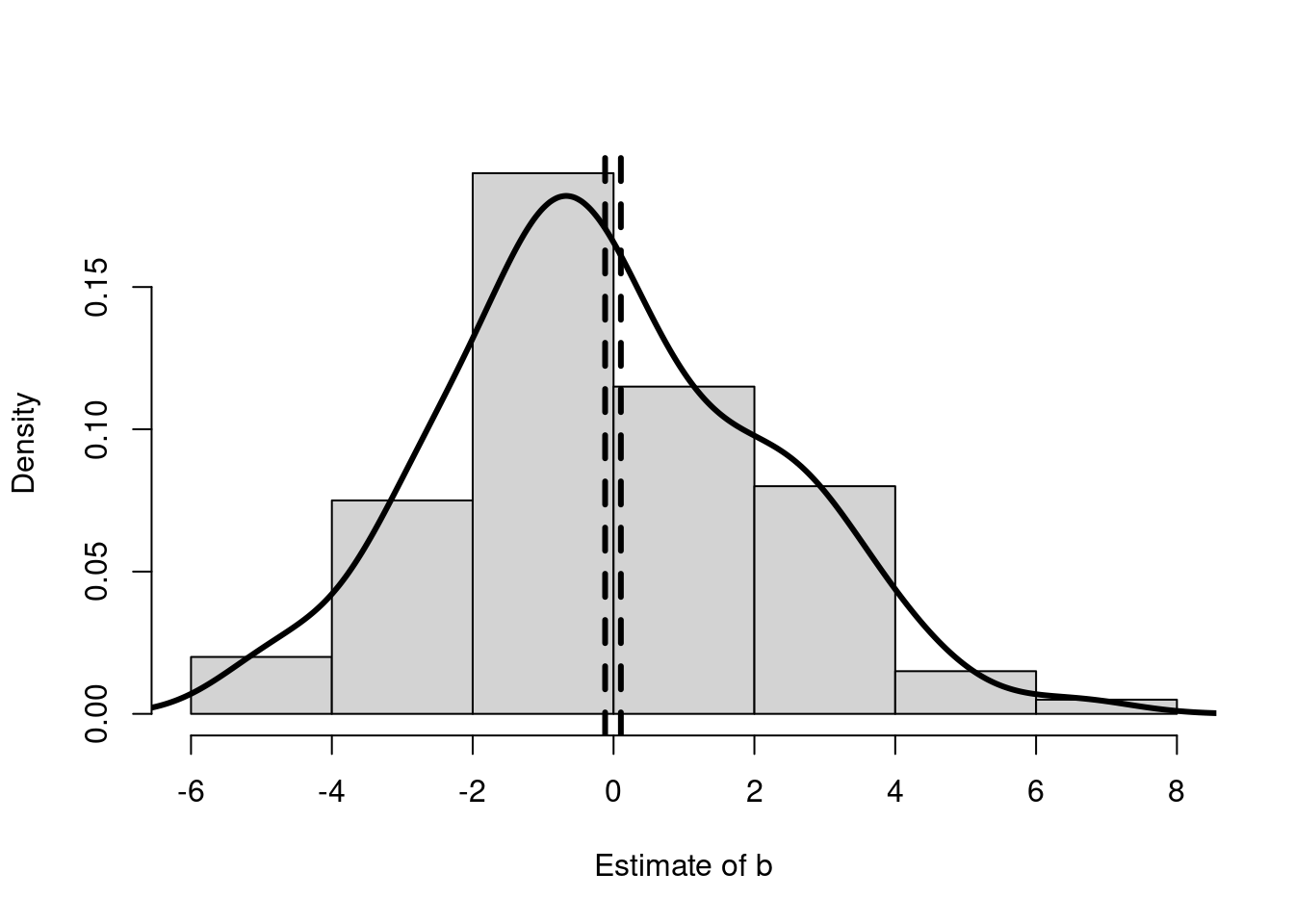
We can use simulation to compare estimators. We rerun the simulation 100 times and summarize the results of the two approaches in Table 5.
The table shows that the proposed estimator gives values much closer to 0 than the standard estimator. It also shows that the standard estimator can, at times, provide misleading results. The estimate may suggest that the value of $b$ is not only not 0, but statistically significantly different from 0. In contrast, the proposed estimate provides values that are always close to 0.

The proposed estimator is much more accurate than the standard estimator. Figure 4 shows the large difference in the accuracy of the two estimates. The standard estimates vary from over -5 to 5, while the proposed estimates have a much much smaller variance. Remember the two approaches are estimated on exactly the same data.

Figure 4

Matrix Algebra of the Dual Path Estimator

We can write out the dual path causal model more generally with matrix algebra. To keep things consistent with the OLS presentation, let $Y$ be the outcome of interest and let $X$ be the value or values that may have both a direct and an indirect effect on $Y$. In addition, let $W$ represent the observed characteristics that may mediate the causal effect of $X$ on $Y$.

$$\begin{gathered} \begin{array}{}\text{(11)}& \mathbf{y}=\mathbf{X}\beta +\mathbf{W}\gamma +ϵ \\ \mathbf{W}=\mathbf{X}\mathrm{\Delta }+\mathbf{{\rm Y}}\end{array} \end{gathered}$$

where $\mathbf{y}$ is a $N\times 1$ vector of the outcomes of interest, $\mathbf{X}$ is a $N\times J$ matrix representing the different variables that may be directly or indirectly determining the outcome, $\mathbf{W}$ is a $N\times K$ matrix representing the variables that are mediating the causal effect of the $X$s on $Y$. The parameters of interest are $\beta$ representing the direct effect and both $\gamma$ and $\mathrm{\Delta }$ representing the indirect effect. Note that while $\beta$ and $\gamma$ are $J\times 1$ and $K\times 1$ vectors respectively, $\mathrm{\Delta }$ is a $J\times K$ matrix representing all the different effects of $\mathbf{X}$ on $\mathbf{W}$. Similarly $ϵ$ is the $N\times 1$ vector of unobserved characteristics affecting the outcome and $\mathbf{{\rm Y}}$ is a $N\times K$ matrix of all the unobserved characteristics determining the different elements of $\mathbf{W}$.

The (Equation 11) presents the model of the data generating process. In the simultaneous equation system we see that the matrix $\mathbf{X}$ enters both directly into the first equation and indirectly through the second equation. Note that the second equation is actually a set of equations representing all the different effects that the values represented by $X$ have on the values represented by $W$. In addition, the unobserved characteristics that affect $\mathbf{y}$ are independent of unobserved characteristics that affect $\mathbf{W}$.

We are interested in estimating $\beta$, but we have learned above that the short regression of $Y$ on $X$ will give the wrong answer and the long regression of $Y$ on $X$ and $W$ will also give the wrong answer. The solution is to estimate $\tilde{\beta }$ which represents the vector of coefficients from the short regression of $Y$ on $X$. Then remember that we can derive $\beta$ by estimating $\mathrm{\Delta }$ and $\gamma$, as $\beta =\tilde{\beta }-\mathrm{\Delta }\gamma$.

All three vectors can be estimated following the same matrix algebra we presented for estimating OLS.

$$\begin{array}{}\text{(12)}& \begin{array}{ll}\hat{\tilde{\beta }}& =({\mathbf{X}}^{\prime }\mathbf{X}{)}^{-1}{\mathbf{X}}^{\prime }\mathbf{y}\\ \hat{\mathrm{\Delta }}& =({\mathbf{X}}^{\prime }\mathbf{X}{)}^{-1}{\mathbf{X}}^{\prime }\mathbf{W}\\ \hat{\gamma }& =({\mathbf{W}}^{\prime }\mathbf{W}{)}^{-1}{\mathbf{W}}^{\prime }\mathbf{y}\end{array}\end{array}$$

The first equation $\hat{\tilde{\beta }}$ represents the “total effect” of the $X$s on $Y$. It is the short regression of $Y$ on $X$. The second equation follows from “dividing” by $\mathbf{X}$ in the second line of (Equation 11). The third equation is the short regression of $Y$ on $W$.

Substituting the results of the last two regressions into the appropriate places we get our proposed estimator for the direct effect of $X$ on $Y$.

$$\begin{array}{}\text{(13)}& \hat{\beta }=({\mathbf{X}}^{\prime }\mathbf{X}{)}^{-1}{\mathbf{X}}^{\prime }\mathbf{y}-({\mathbf{X}}^{\prime }\mathbf{X}{)}^{-1}{\mathbf{X}}^{\prime }\mathbf{W}({\mathbf{W}}^{\prime }\mathbf{W}{)}^{-1}{\mathbf{W}}^{\prime }\mathbf{y}\end{array}$$

The (Equation 13) presents the estimator of the direct effect of the $X$s on $Y$. Note that our proposed estimate of $\gamma$ may be biased if the direct effect of $X$ on $Y$ is non-zero.¹²

Dual Path Estimator in R

The (Equation 13) is pseudo-code for the dual-path estimator in R.

X <- cbind(1,x)
W <- cbind(1,w)
beta_tilde_hat <- solve(t(X)%*%X)%*%t(X)%*%y 
Delta_hat <- solve(t(X)%*%X)%*%t(X)%*%W
gamma_hat <- solve(t(W)%*%W)%*%t(W)%*%y
beta_tilde_hat - Delta_hat%*%gamma_hat

         [,1]
  -0.01515376
x  0.02444155

The estimated value of $\hat{\beta }=\{-0.015,0.024\}$ is pretty close to the true value of $\beta =\{0,0\}$.

Are Bankers Racist or Greedy?

African Americans are substantially more likely to be denied mortgages than whites. Considering data used by Munnell et al. (1996), being black is associated with a 20% reduction in the likelihood of getting a mortgage.¹³ The US Consumer Financial Protection Bureau states that the Fair Housing Act may make it illegal to refuse credit based on race.¹⁴

Despite these observed discrepancies, lenders may not be doing anything illegal. It may not be illegal to deny mortgages based on income or credit history. Bankers are allowed to maximize profits. They are allowed to deny mortgages to people that they believe are at high risk of defaulting. There may be observed characteristics of the applicants that are associated with a high risk of defaulting that are also associated with race.

Determining the causal pathway has implications for policy. If the effect of race is direct, then laws like the Fair Housing Act may be the correct policy response. If the effect is indirect, then such a policy will have little effect on a policy goal of increasing housing ownership among African Americans.

The section finds that there may be no direct effect of race on mortgage lending.

Boston HMDA Data

The data used here comes from Munnell et al. (1996). This version is downloaded from the data sets for Stock and Watson (2011) here: https://wps.pearsoned.com/aw_stock_ie_3/178/45691/11696965.cw/index.html. You can also download a csv version of the data from https://sites.google.com/view/microeconometricswithr/table-of-contents.

x <- read.csv("hmda_aer.csv", as.is = TRUE) 
x$deny <- ifelse(x$s7==3,1,NA)
# ifelse considers the truth of the first element.  If it is 
# true then it does the next element, if it is false it does
# the final element.
# You should be careful and make sure that you don't 
# accidentally misclassify an observation.  
# For example, classifying "NA" as 0.
# Note that == is used in logical statments for equal to.
x$deny <- ifelse(x$s7==1 | x$s7==2,0,x$deny)
# In logical statements | means "or" and & means "and".
# The variable names refer to survey questions.  
# See codebook.
x$black <- x$s13==3 # we can also create a dummy by using 
# true/false statement.

The following table presents the raw effect of race on mortgage denials from the Munnell et al. (1996) data. It shows that being African American reduces the likelihood of a mortgage by 20 percentage points.

Table 6: OLS results of mortgage denials on race using data from Munnell et al. (1996).

Estimate Std. Error t value Pr(>|t|) (Intercept) 0.1131461 0.0069434 16.29557 0 blackTRUE 0.1945462 0.0173584 11.20760 0

Causal Pathways of Discrimination

Race may be affecting the probability of getting a mortgage through two different causal pathways. There may be a direct effect in which the lender is denying a mortgage because of the applicant’s race. There may be an indirect effect in which the lender denies a mortgage based on factors such as income or credit history. Race is associated with lower income and poorer credit histories.

Figure 5: Dual path causal graph of mortgage denials.

Figure 5 represents the estimation problem. The regression in Table 6 may be picking up both the direct effect of Race on Deny ($b$) and the indirect effect of Race on Deny mediated by Income ($dc$).

Estimating the Direct Effect

x$lwage <- NA
x[x$s31a>0 & x$s31a<999999,]$lwage <- 
  log(x[x$s31a>0 & x$s31a<999999,]$s31a)
# another way to make sure that NAs are not misclassified.
# See the codebook for missing data codes.
x$mhist <- x$s42
x$chist <- x$s43
x$phist <- x$s44
x$emp <- x$s25a
x$emp <- ifelse(x$emp>1000,NA,x$emp)

To determine the causal effect of race we can create a number of variables from the data set that may mediate race. These variables measure information about the applicant’s income, employment history and credit history.

Y1 <- x$deny
X1 <- cbind(1,x$black)
W1 <- cbind(1,x$lwage,x$chist,x$mhist,x$phist,x$emp)
index <- is.na(rowSums(cbind(Y1,X1,W1)))==0 
# this removes missing values.
X2 <- X1[index,]
Y2 <- Y1[index]
W2 <- W1[index,]
beta_tilde_hat <- solve(t(X2)%*%X2)%*%t(X2)%*%Y2 
Delta_hat <- solve(t(X2)%*%X2)%*%t(X2)%*%W2
gamma_hat <- solve(t(W2)%*%W2)%*%t(W2)%*%Y2
beta_tilde_hat - Delta_hat%*%gamma_hat

            [,1]
[1,] -0.01797654
[2,]  0.11112066

Adding these variables reduces the possible direct effect of race on mortgage denials by almost half. Previously, the analysis suggested that being African American reduced the probability of getting a mortgage by 20 percentage points. This analysis shows that at least 8 percentage points of that is due to an indirect causal effect mediated by income, employment history, and credit history. Can adding in more such variables reduce the estimated direct causal effect of race to zero?

Adding in More Variables

x$married <- x$s23a=="M"  
x$dr <- ifelse(x$s45>999999,NA,x$s45)
x$clines <- ifelse(x$s41>999999,NA,x$s41)
x$male <- x$s15==1
x$suff <- ifelse(x$s11>999999,NA,x$s11)
x$assets <- ifelse(x$s35>999999,NA,x$s35)
x$s6 <- ifelse(x$s6>999999,NA,x$s6)
x$s50 <- ifelse(x$s50>999999,NA,x$s50)
x$s33 <- ifelse(x$s33>999999,NA,x$s33)
x$lr <- x$s6/x$s50
x$pr <- x$s33/x$s50
x$coap <- x$s16==4
x$school <- ifelse(x$school>999999,NA,x$school)
x$s57 <- ifelse(x$s57>999999,NA,x$s57)
x$s48 <- ifelse(x$s48>999999,NA,x$s48)
x$s39 <- ifelse(x$s39>999999,NA,x$s39)
x$chval <- ifelse(x$chval>999999,NA,x$chval)
x$s20 <- ifelse(x$s20>999999,NA,x$s20)
x$lwage_coap <- NA
x[x$s31c>0 & x$s31c < 999999,]$lwage_coap <- 
  log(x[x$s31c>0 & x$s31c < 999999,]$s31c)
x$lwage_coap2 <- ifelse(x$coap==1,x$lwage_coap,0)
x$male_coap <- x$s16==1

We can add in a large number of variables that may be reasonably associated with legitimate mortgage denials, including measures of assets, ratio of debt to assets and property value. Lenders may also plausibly deny mortgages based on whether the mortgage has a co-applicant and characteristics of the co-applicant.

W1 <- cbind(1,x$lwage,x$chist,x$mhist,x$phist,x$emp,
            x$emp^2,x$married,x$dr,x$clines,x$male,
            x$suff,x$assets,x$lr,x$pr,x$coap,x$s20,
            x$s24a,x$s27a,x$s39,x$s48,x$s53,x$s55,x$s56,
            x$s57,x$chval,x$school,x$bd,x$mi,x$old,
            x$vr,x$uria,x$netw,x$dnotown,x$dprop,
            x$lwage_coap2,x$lr^2,x$pr^2,x$clines^2,x$rtdum)
# x$rtdum measures the racial make up of the neighborhood.
index <- is.na(rowSums(cbind(Y1,X1,W1)))==0 
X2 <- X1[index,]
Y2 <- Y1[index]
W2 <- W1[index,]

Bootstrap Dual Path Estimator in R

The bootstrap estimator uses the algebra as pseudo-code for an estimator in R.

set.seed(123456789)
K <- 1000
bs_mat <- matrix(NA,K,2)
for (k in 1:K) {
  index_k <- round(runif(length(Y2),min=1,max=length(Y2)))
  Y3 <- Y2[index_k]
  X3 <- X2[index_k,]
  W3 <- W2[index_k,]
  beta_tilde_hat <- solve(t(X3)%*%X3)%*%t(X3)%*%Y3
  Delta_hat <- solve(t(X3)%*%X3)%*%t(X3)%*%W3
  gamma_hat <- solve(t(W3)%*%W3)%*%t(W3)%*%Y3
  bs_mat[k,] <- beta_tilde_hat - Delta_hat%*%gamma_hat
  # print(k)
}
tab_res <- matrix(NA,2,4)
tab_res[,1] <- colMeans(bs_mat)
tab_res[,2] <- apply(bs_mat, 2, sd)
tab_res[1,3:4] <- quantile(bs_mat[,1], c(0.025,0.975))
# first row, third and fourth column.
tab_res[2,3:4] <- quantile(bs_mat[,2], c(0.025,0.975))
colnames(tab_res) <- c("Estimate", "SD", "2.5%", "97.5%")
rownames(tab_res) <- c("intercept","direct effect")

kable(tab_res)

Table 7: Bootstrapped estimates of the proposed approach to estimating the direct effect of race on mortgage denials.

	Estimate	SD	2.5%	97.5%
intercept	-0.0036116	0.0026838	-0.0089441	0.0017112
direct effect	0.0236503	0.0176671	-0.0108709	0.0580450

Adding in all these variables significantly reduces the estimate of the direct effect of race on mortgage denials. The estimated direct effect of being African American falls from a 20 percentage point reduction in the probability of getting a mortgage to a 2 percentage point reduction. A standard hypothesis test with bootstrapped standard errors states that we cannot rule out the possibility that the true direct effect of race on mortgage denials is zero.¹⁵

Policy Implications of Dual Path Estimates

The analysis shows that African Americans are much more likely to be denied mortgages in Boston during the time-period. If this is something a policy maker wants to change, then she needs to know why African Americans are being denied mortgages. Is it direct discrimination of the banks? Or is the effect indirect because African Americans tend to have lower income and poorer credit ratings than other applicants. A policy that makes it illegal to use race directly in mortgage decisions will be more effective if bankers are in fact using race directly in mortgage decisions. Other policies may be more effective if bankers are using credit ratings and race is affecting loan rates indirectly.

Whether this analysis answers the question is left to the reader. It is not clear we should include variables such as the racial make up of the neighborhood or the gender of the applicant. The approach also relies on the assumption that there is in fact no direct effect of race on mortgage denials. In addition, it uses OLS rather than models that explicitly account for the discrete nature of the outcome variable.¹⁶

The approach presented here is quite different from the approach presented in Munnell et al. (1996). The authors are also concerned that race may have both direct and indirect causal effects on mortgage denials. Their solution is to estimate the relationship between the mediating variables ($W$) and mortgage denials ($Y$). In Figure 5 they are estimating $c$. The authors point out that the total effect of race on mortgage denials is not equal to $c$. They conclude that bankers must be using race directly. The problem is that they only measured part of the indirect effect. They did not estimate $d$. That is, their proposed methodology does not answer the question of whether bankers use race directly.

Discussion and Further Reading

There is a simplistic idea that longer regressions must be better than shorter regressions. The belief is that it is always better to add more variables. Hopefully, this chapter showed that longer regressions can be better than shorter regressions, but they can also be worse. In particular, long regressions can create multicollinearity problems. While it is funny, Goldberger’s chapter on multicollinearity downplays the importance of the issue.

The chapter shows that if we take DAGs seriously we may be able to use an alternative to the long regression. The chapter shows that in the case where there are two paths of a causal effect, we can improve upon the long regression. I highly recommend Pearl and Mackenzie (2018) to learn more about graphs. Pearl uses the term “mediation” to refer to the issue of dual causal paths.

To find out more about the lawsuit against Harvard University, go to https://studentsforfairadmissions.org/.

References

Card, David. 1995. “Aspects of Labour Market Behavior: Essays in Honour of John Vanderkamp.” In, edited by Louis N. Christofides, E. Kenneth Grant, and Robert Swidinsky, 201–22. University of Toronto Press.

Goldberger, Arthur. 1991. A Course in Econometrics. Harvard University Press.

Hlavac, Marek. 2018. “Stargazer: Well-Formatted Regression and Summary Statistics Tables.”

Munnell, Alicia H., Geoffrey M. B. Tootell, Lynn E. Brown, and McEneaney. 1996. “Mortgage lending in Boston: interpreting HMDA data.” The American Economic Review 86 (1): 25–53.

Pearl, Judea, and Dana Mackenzie. 2018. The Book of Why: The New Science of Cause and Effect. Basic Books.

Stock, James H, and Mark W Watson. 2011. Introduction to Econometrics. Third. Pearson.

Footnotes

1. Actually, the combined effect is captured by adding the two coefficients together. The model can’t separate the two effects.

2. The table uses the stargazer package (Hlavac 2018). If you are using stargazer in Sweave then start the chunk with results=tex embedded in the chunk header.

3. Matrix rank refers to the number of linearly independent columns or rows.

4. Micronumerosity refers to the problem of small sample size.

5. As an exercise try to replicate the whole table. Note that you will need to carefully read the discussion of how the various variables are created.

6. See discussion in Chapter 1 regarding interpreting the coefficient.

7. The UCLA computer scientist, Judea Pearl, is a proponent of using DAGs in econometrics. These diagrams are models of how the data is generated. The associated algebra helps the econometrician and the reader determine the causal relationships and whether or not they can be estimated (Pearl and Mackenzie 2018).

8. https://studentsforfairadmissions.org/

9. It is the reciprocal of $d$ because we follow the arrow backwards from $W$ to $X$.

10. You should think about the reasonableness of this assumption for the problem discussed below.

11. See discussion of hypothesis testing in Appendix A.

12. See earlier discussion.

13. The code book for the data set is located here: https://sites.google.com/view/microeconometricswithr/table-of-contents

14. https://www.consumerfinance.gov/fair-lending/

15. See discussion of hypothesis testing in Appendix A.

16. It may more appropriate to use a probit or logit. These models are discussed in Chapter 5.