Demand Estimation with IV

Introduction

When I began teaching microeconometrics a few years ago I read up on the textbook treatment of demand estimation. There was a lot of discussion about estimating logits and about McFadden’s model. It looked a lot like how I was taught demand estimation 25 years before. It looked nothing like the demand estimation that I have been doing for the last 20 years. Demand estimation is integral to antitrust analysis. It is an important part of marketing and business strategy. But little of it actually involves estimating a logit. Modern demand estimation combines the insights of instrumental variable estimation and game theory.

My field, industrial organization, changed dramatically in the 1970s and 1980s as game theory became the major tool of analysis. A field that had been dominated by industry studies quickly became the center of economic theory and the development of game theoretic analysis in economics. By the time I got to grad school in the mid 1990s, the field was changing again. New people were looking to combine game theory with empirical analysis. People like Susan Athey, Harry Paarsh and Phil Haile started using game theory to analyze timber auctions and oil auctions. Others like Steve Berry and Ariel Pakes were taking game theory to demand estimation.

Game theory allows the econometrician to make inferences from the data by theoretically accounting for the way individuals make decisions and interact with each other. As with discrete choice models and selection models, we can use economic theory to help uncover unobserved characteristics. Again, we assume that economic agents are optimizing. The difference here is that we allow economic agents to explicitly interact and we attempt to model that interaction. Accounting for such interactions may be important when the number of agents is small and it is reasonable to believe that these individuals do in fact account for each others’ actions.

This chapter presents a standard model of competition, the Hotelling model. It presents two IV methods for estimating demand from simulated data generated by the Hotelling model. It introduces the idea of using both cost shifters and demand shifters as instruments. The chapter takes these tools to the question of estimating the value of Apple Cinnamon Cheerios.

Modeling Competition

In the late 1920s, the economist and statistician, Harold Hotelling, developed a model of how firms compete. Hotelling wasn’t interested in “perfect competition,” and its assumption of many firms competing in a market with homogeneous products. Hotelling was interested in what happened when the number of firms is small and the products are similar but not the same. Hotelling (1929) was responding to an analysis written the French mathematician, Joseph Bertrand, some 80 years earlier. Bertrand, in turn, was responding to another French mathematician, Antoine Cournot, whose initial analysis was published in the 1830s.

All three were interested in what happens when two firms compete. In Cournot’s model, the two firms make homogeneous products. They choose how much to produce and then the market determines the price. Cournot showed that this model leads to much higher prices than was predicted by the standard (at the time) model of competition. Bertrand wasn’t convinced. Bertrand considers the same case but had the firms choose prices instead.

Imagine two hotdog stands next to each other. They both charge $2.00 a hotdog. Then one day, the left stand decides to charge $1.90 a hotdog. What do you think will happen? When people see that the left stand is charging $1.90 and the right one is charging $2.00, they are likely to buy from the left one. Seeing this, the right hotdog stand reacts and sets her price at $1.80 a hotdog. Seeing the change, everyone switches to the right stand. Bertrand argued that this process will lead prices to be bid down to marginal cost. That is, with two firms the model predicts that prices will be the same as the standard model.

Hotelling agreed that modeling the firms as choosing price seemed reasonable, but was unconvinced by Bertrand’s argument. Hotelling suggested a slight change to the model. Instead of the two hotdog stands being next to each other, he placed them at each end of the street. Hotelling pointed out that in this case even if the left stand was 10c cheaper, not everyone would switch away from the right stand. Some people have their office closer to the right stand and are unwilling to walk to the end of the street just to save a few cents on their hotdog. Hotelling showed that in this model prices were again much higher than for the standard model.

When I think about competition, it is Hotelling’s model that I have in my head.

Competition is a Game

Hotelling, Cournot and Bertrand all modeled competition as a game. A game is a formal mathematical object which has three parts; players, strategies and payoffs. In the game considered here, the players are the two firms. The strategies are the actions that the players can take given the information available to them. The payoffs are the profits that the firms make. Note that in Cournot’s game, the strategy is the quantity that the firm chooses to sell. In Bertrand’s game, it is the price that the firm chooses to sell at. Cournot’s model is a reasonable representation of an exchange or auction. Firms decide how much to put on the exchange and prices are determined by the exchange’s mechanism. In Bertrand’s game, the firm’s post prices and customers decide how much to purchase.

Table 1: A pricing game where Firms 1 and 2 choose prices $\{p_{jL},p_{jH}\}$.

$\{F_1,F_2\}$	$p_{2L}$	$p_{2H}$
$p_{1L}$	{1,1}	{3,0}
$p_{1H}$	{0,3}	{2,2}

Consider the following pricing game represented in Table Table 1. There are two firms, Firm 1 and Firm 2. Each firm chooses a price, either $p_L$ or $p_H$. The firm’s profits are in the cells. The first number refers to the profit that Firm 1 receives.

What do you think will be the outcome of the game? At which prices do both firms make the most money? If both firms choose $p_H$ the total profits will be 4, which is split evenly. Will this be the outcome of the game?

No. At least it won’t be the outcome if the outcome is a Nash equilibrium. The outcomes of the games described by Hotelling, Bertrand and Cournot are all Nash equilibrium. Interestingly, John Nash, didn’t describe the equilibrium until many years later, over 100 years later in the case of Bertrand and Cournot. Even the definition of a game didn’t come into existence until the work of mathematicians like John von Neumann in the early 20th century.

A Nash equilibrium is where each player’s strategy is optimal given the strategies chosen by the other players. Here, a Nash equilibrium is where Firm 1’s price is optimal given Firm 2’s price, and Firm 2’s price is optimal given Firm 1’s price. It is not a Nash equilibrium for both firms to choose $p_H$. If Firm 2 chooses $p_{2H}$, then Firm 1 should choose $p_{1L}$ because the payoff is 3, which is greater than 2. Check this by looking at the second column of the table and the payoffs for Firm 1, which are the first element of each cell.

The Nash equilibrium is $\{p_{1L},p_{2L}\}$. You can see that if Firm 2 chooses $p_{2L}$, then Firm 1 earns 1 from also choosing $p_{1L}$ and 0 from choosing $p_{2H}$. The same argument can be made for Firm 2 when Firm 1 chooses $p_{1L}$. Do you think this outcome seems reasonable?

Hotelling’s Line

Figure 1: Hotelling’s line with Firm $L$ located at 0 and Firm $R$ located at 1. Everyone “living” left of $x_L$ purchases from Firm $L$.

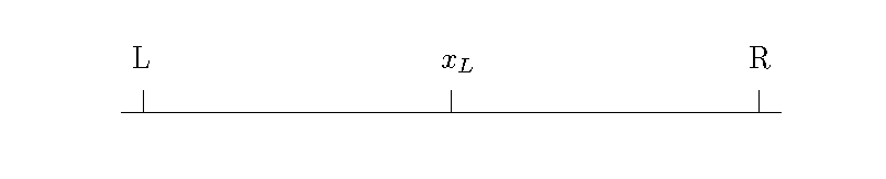
The Figure 1 represents Hotelling’s game. There are two firms $L$ and $R$. Customers for the two firms “live” along the line. Customers prefer to go to the closer firm if the products and prices are otherwise the same. Hotelling’s key insight is that while firms often compete by selling similar products, these products may not be identical. Moreover, some people may prefer one product to the other. Some people actually prefer Pepsi to Coke or 7Up to Sprite. The location on the line represents how much certain customers prefer $L$ to $R$.

Let Firm $L$ lie at 0 and Firm $R$ lie at 1. An infinite number of customers are located between 0 and 1. This infinite number of customers has a mass of 1. That is, we can think of location as a probability of purchasing from Firm $L$. Consider the utility of a customer at location $x\in [0,1]$. This customer buys from $L$ if and only if the following inequality holds.

$$\begin{array}{}\text{(1)}& U_L=v_L-x-\beta p_L>v_R-(1-x)-\beta p_R=U_R\end{array}$$

where $v_L$ and $v_R$ are the value of $L$ and $R$ respectively, $p_L$ and $p_R$ are the prices and $\beta$ represents how customers relate the product to prices. The customer located at $x_L$ is indifferent between buying from $L$ or $R$.

$$\begin{array}{}\text{(2)}& \begin{array}{l}v-x_L-\beta (p_L-p_R)=-1+x_L\\ x_L=\frac{v+1-\beta p_L+\beta p_R}{2}\end{array}\end{array}$$

where $v=v_L-v_R$. This is also the demand for Firm $L$.

Everyone located between 0 and $x_L$ will buy from Firm $L$. Everyone on the other side will buy from Firm $R$. Given that everyone buys 1 unit, the demand for Firm $L$’s product is $x_L$ and demand for Firm $R$’s product is $1-x_L$.

Nash Equilibrium

Given all this, what will be the price in the market? We assume that the price is determined by the Nash equilibrium. Each firm is assumed to know the strategy of the other firm. That is, each firm knows the price of their competitor. The Nash equilibrium is the price such that Firm $L$ is unwilling to change their price given the price charged by Firm $R$, and Firm $R$ is unwilling to change their price given Firm $L$’s price.

Firm L’s problem is as follows.

$$\begin{array}{}\text{(3)}& ma{x}_{p_L}\frac{(v+1-\beta p_L+\beta p_R)(p_L-c_L)}{2}\end{array}$$

where $c_L$ is the marginal cost of $L$. Firm $L$’s profits are equal to its demand ($x_L$) multiplied by its markup, price less marginal cost($p_L-c_L$).

The solution to the optimization problem is the solution to the first order condition.

$$\begin{array}{}\text{(4)}& \frac{v+1-\beta p_L+\beta p_R}{2}-\frac{\beta p_L-\beta c_L}{2}=0\end{array}$$

Firm R’s problem is similar.

$$\begin{array}{}\text{(5)}& ma{x}_{p_R}\frac{(-v-1+\beta p_L-\beta p_R)(p_R-c_R)}{2}\end{array}$$

The first order condition is as follows.

$$\begin{array}{}\text{(6)}& \frac{-v-1+\beta p_L-\beta p_R}{2}-\frac{\beta p_R-\beta c_R}{2}=0\end{array}$$

Given these first order conditions we can write down a system of equations.

$$\begin{array}{}\text{(7)}& \begin{array}{l}{p}_L=\frac{v+1+\beta p_R+\beta c_L}{2\beta }\\ \\ p_R=\frac{-v-1+\beta p_L+\beta c_R}{2\beta }\end{array}\end{array}$$

Solving the system we have the Nash equilibrium prices in the market.

$$\begin{array}{}\text{(8)}& \begin{array}{l}{p}_L=\frac{v+1+\beta c_R+2\beta c_L}{3\beta }\\ \\ p_R=\frac{-v-1+\beta c_L+2\beta c_R}{3\beta }\end{array}\end{array}$$

In equilibrium, prices are determined by the relative value of the products ($v$), the willingness to switch between products based on price ($\beta$) and marginal costs ($c_L$ and $c_R$). Note that Firm $L$’s price is determined by Firm $R$’s marginal costs. Do you see why that would be?

Estimating Demand in Hotelling’s Model

We can illustrate the modern approach to demand estimation using Hotelling’s model. The section creates a simulated the demand system based on the model and estimates the parameters using the IV approach.

Simulation of Hotelling Model

The simulation uses the model above to create market outcomes including prices and market shares. There are 1,000 markets. These may represent the two firms competing at different times or different places. The data is adjusted to keep market outcomes where prices are positive and shares are between 0 and 1.

set.seed(123456789)
N <- 1000 # number of markets
beta = 0.25 # demand parameter
v <- 3 + rnorm(N) # quality (vertical) measure
cL <- 3 + rnorm(N)
cR <- 9 + rnorm(N)
# costs for both firms.
pL <- (v + 1 + beta*cR  + 2*beta*cL)/(3*beta)
pR <- (-v - 1 + beta*cL + 2*beta*cR)/(3*beta)
# price function for each firm.
xL <- (v + 1 - beta*pL + beta*pR)/2
# demand for firm L
index <- pL > 0 & pR > 0 & xL > 0 & xL < 1
cL1 <- cL[index]
cR1 <- cR[index]
pL1 <- pL[index]
pR1 <- pR[index]
xL1 <- xL[index]
v1 <- v[index]
# adjusting values to make things nice.

Figure 2: Demand for Firm L by relative price of Firm L to Firm R.

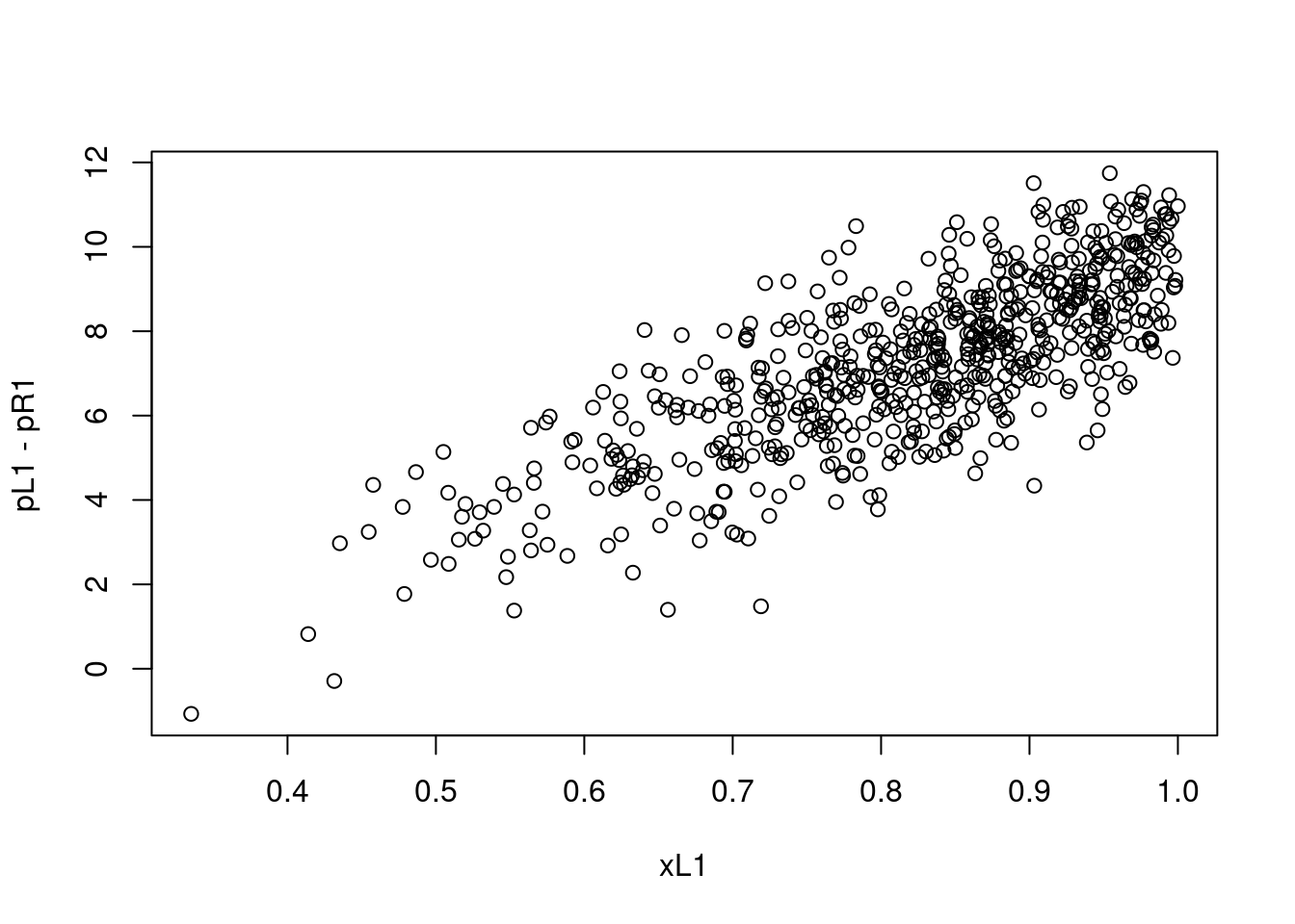
The Figure 2 plots demand and relative price for product $L$ from the simulated data. Do you notice anything odd about the figure? Remembering back to Econ 101, did demand slope up or down? It definitely slopes down in Equation 2. What went wrong?

Prices are Endogenous

Probably every economist in industrial organization has run a regression like what is depicted in Figure 2. Each one has looked at the results and has felt their heart sink because everything that they knew about economics was wrong. Then they have taken a deep breath and remembered prices are endogenous.

We are interested in estimating how prices affect demand for the product. We know they do. Equation 2 explicitly states that prices cause demand to fall. The problem is that we did not plot the demand curve. We plotted out a bunch of outcomes from the market. We plotted out a thousand equilibrium prices and equilibrium demand levels. Back to Econ 101, think of a thousand demand and supply crosses going through each of the points in Figure 2.

The problem in the simulation is that prices are determined endogenously. The observed market prices are the outcome of the Nash equalibria and the choices of Firm $L$ and Firm $R$. If we want to estimate the demand for Firm $L$ (Equation 2) then one approach is to use the instrumental variables methods discussed in Chapter 3.

Cost Shifters

The standard instrumental variable approach is to use cost shifters. That is, we need an instrument related to costs. For example, if we observed $c_L$ in the simulated data, then that would work as instrument. It satisfies the assumptions. It has a direct effect on $p_L$ through Equation 8. It does not direct affect $x_L$, see Equation 2.

# Intent to Treat
lm1 <- lm(xL1 ~ I(cL1-cR1))
# First stage
lm2 <- lm(I(pL1-pR1) ~ I(cL1-cR1))
# IV estimate
lm1$coefficients[2]/lm2$coefficients[2]

I(cL1 - cR1) 
 -0.04755425 

Remember back to Chapter 3, we can use graph algebra to find a simple estimator. This is the intent to treat regression (demand on costs) divided by the first stage regression (price on costs). Note that price of interest is the difference in the prices of the two firms. The instrument for this price is the difference in the costs of the two firms. The estimate is -0.048. The true value is -0.125, which you see from Equation 2 where $\beta =0.25$ and the price effect is $\frac{-\beta }{2}$. It is not particularly accurate, but at least it is negative!

X1 <- cbind(pL1,pR1)
Z1 <- cbind(cL1,cR1)
Y1 <- as.matrix(xL1)
tab_ols <- lm_iv(Y1,X1, Reps=500)
tab_iv <- lm_iv(Y1, X1, Z1, Reps = 500)
# using the function defined in chapter 3.
row.names(tab_iv) <- row.names(tab_ols) <- 
  c("intercept",colnames(X1))
tab_res <- cbind(tab_ols[,1:2],tab_iv[,1:2])
colnames(tab_res) <- 
  c("OLS coef","OLS sd","IV coef", "IV sd")

library(knitr)

kable(tab_res)

Table 2: OLS and IV bootstrapped estimates of demand for the Hotelling model.

	OLS coef	OLS sd	IV coef	IV sd
intercept	0.5086192	0.0265343	1.1012163	0.0981138
pL1	0.0446127	0.0024228	-0.0428697	0.0116172
pR1	-0.0491404	0.0027078	0.0547691	0.0140925

We can also use the matrix algebra method described in Chapter 3. Here we separate out the two prices and don’t use the information that they have the same coefficient. We can confirm the results of Figure 2; relationship between price and demand have the wrong sign. The IV estimate is again on the low side at around -0.04.

Demand Shifters

The analysis above is the standard approach to IV in demand analysis. However, we are not limited to using cost shifters. In the simulation there is a third exogenous variable, $v$. This variable represents factors that make Firm $L$’s product preferred to Firm $R$’s product. We call this a vertical difference as opposed to the location along the line which we call horizontal. In the real world a vertical difference may refer to the quality of the product. Everyone prefers high quality products.

Looking at the Nash equilibrium (Equation 8), we see that $v$ positively affects the price that Firm $L$ charges. The variable increases demand which allows the firm to charge higher prices. But this is not what we are interested in. Our goal is to estimate the slope of the demand curve. We can use the model to determine the value of interest. Equation 8 provides the relationship between $p_L$ and $v$ which is equal to $\frac{1}{3\beta }$, while the slope of demand is $-\frac{\beta }{2}$. We can use the first to determine the second. This gives -0.116, which is pretty close to -0.125. In fact, this method does better than the more standard approach.

lm1 <- lm(pL1 ~ v1)
b1 <- lm1$coefficients[2]
beta <- 1/(3*b1)
-beta/2

        v1 
-0.1162436 

The idea of using the model in this way is at the heart of much of modern industrial organization. The idea is to use standard statistical techniques to estimate parameters of the data, and then use the model to relate those data parameters to the model parameters of interest. The idea was promoted by Guerre, Perrigne, and Vuong (2000) who use an auction model to back out the underlying valuations from observed bids.¹

Berry Model of Demand

Yale industrial organization economist, Steve Berry, is probably the person most responsible for the modern approach to demand analysis. S. Berry, Levinsohn, and Pakes (1995) may be the most often used method in IO. We are not going to unpack everything in that paper. Rather, we will concentrate on the two ideas of demand inversion and taking the Nash equilibrium seriously.

We are interested in estimating demand. That is, we are interested in estimating the causal effect of price ($p$) on demand (or share) ($s$). A firm would like to know what would happen to its demand if it increases the price 10%. Will its revenue increase or decrease? In the earlier sections, variation in prices or other characteristics of the product are used to infer demand. The problem is that prices may not be exogenously determined.

This section presents a general IV approach to demand estimation.

Choosing Prices

To see how marginal costs affect price consider a simple profit maximizing firm $j$ with constant marginal cost ($c_j$). Demand for the firm’s product is denoted $s(p_j,p_{-j})$ (share), where $p_i$ is their own price and $p_{-j}$ are the prices of the competitors in the market ($-j$ means not $j$). The firm’s pricing decision is based on maximizing its profit function.

$$\begin{array}{}\text{(9)}& \begin{array}{ll}\underset{p_j}{max}& s_j(p_j,p_{-j})(p_j-c_j)\end{array}\end{array}$$

The Equation 9 shows a firm choosing prices to maximize profits, which is quantity times margin. The solution to the maximization problem can be represented as the solution to a first order condition.

$$\begin{array}{}\text{(10)}& s_{j1}(p_j,p_{-j})(p_j-c_j)+s_j(p_j,p_{-j})=0\end{array}$$

where $s_{j1}$ is the derivative with respect to $p_j$. This equation can be rearranged to give the familiar relationship between margins and demand.

$$\begin{array}{}\text{(11)}& \frac{p_j-c_j}{p_j}=-\frac{s_j(p_j,p_{-j})}{p_j{s}_{j1}(p_j,p_{-j})}=-\frac{1}{ϵ(p_j,p_{-j})}\end{array}$$

where $ϵ(p_j,p_{-j})$ represents the elasticity of demand. For a profit maximizing firm, we can write out the optimal price margin as equal to the reciprocal of the elasticity of demand. The more elastic the demand, the lower the firm’s margin.

A Problem with Cost Shifters

The Equation 11 shows that as marginal cost ($c$) increases, price must increase. To see the exact relationship use the Implicit Function Theorem on Equation 10.

$$\begin{array}{}\text{(12)}& \begin{array}{l}\frac{d{p}_j}{d{c}_j}=-\frac{\frac{d.}{d{c}_j}}{\frac{d.}{d{p}_j}}\\ =\frac{s_{j1}(p_j,p_{-j})}{s_{j11}(p_j,p_{-j})(p_j-c_j)+2s_{j1}(p_j,p_{-j})}\end{array}\end{array}$$

where $s_{j11}$ is the second derivative with respect to $p_j$. As $s_{j1}(p_j,p_{-j})<0$ (demand slopes down), prices are increasing in costs. One of the IV assumptions holds, at least in theory. However, for all of the IV assumptions to hold we need linear demand or an equivalent assumption. That is, we need $s_{j11}(p_j,p_{-j})=0$.²

$$\begin{array}{}\text{(13)}& \begin{array}{l}\frac{d{p}_j}{d{c}_j}=\frac{s_{j1}(p_j,p_{-j})}{2s_{j1}(p_j,p_{-j})}\\ =\frac{1}{2}\end{array}\end{array}$$

From Equation 12, this assumption gives a linear relationship between price and marginal cost.

Empirical Model of Demand

Consider a case similar to that discussed in Chapter 5. We observe a large number of “markets” $t$ with various products in each market. In the example below, the markets are supermarkets in particular weeks, and the products are different cereals.

For simplicity assume that there are just two products. The demand for product $j$ in time $t$ is the following share of the market.

$$\begin{array}{}\text{(14)}& s_{tj}=1-F({\mathbf{X}}_{tj}^{\prime }\gamma +\beta p_{tj}+{\xi }_{tj})\end{array}$$

where the share ($s_{tj}$) is the probability that individuals prefer product $j$ to the alternative. The probability distribution is $F$. Inside $F$ is a linear index, which looks like a standard OLS regression. The matrix $\mathbf{X}$ represents observable characteristics of the product, $\gamma$ is a vector of preferences over those products, $p_{tj}$ is the price of the product, $\beta$ the preference of price and ${\xi }_{tj}$ represents unobserved characteristics of the product.

This model is similar to the logit and probit models presented in Chapter 5. More formally, the model assumes that utility is quasi-linear. In this case, the assumption allows a neat trick. If we can invert $F$ (and we usually can), we can write firm prices as a nice linear function of the $X$s.

Inverting Demand

Instead of writing demand as a function of price, we can write price as a function of demand.

$$\begin{array}{}\text{(15)}& p_{tj}=\frac{-{\mathbf{X}}_{tj}^{\prime }\gamma }{\beta }-\frac{{\xi }_{tj}}{\beta }+\frac{F^{-1}(1-s_{tj})}{\beta }\end{array}$$

The inversion provides a nice linear relationship between price, the index over product characteristics and the inverse of the market share. Now that things are linear we can use standard IV methods. Unfortunately, things get a lot more complicated with more choices. It is not even clear that this “inversion” is always possible (S. T. Berry, Gandhi, and Haile 2013).

In the special case of the logit demand, things are relatively straightforward (S. Berry 1994).

$$\begin{array}{}\text{(16)}& s_{tj}=\frac{\exp ({\mathbf{X}}_{tj}^{\prime }\gamma +\beta p_{tj}+{\xi }_{tj})}{1+\sum _{k=1}^J\exp ({\mathbf{X}}_{tk}^{\prime }\gamma +\beta p_{tk}+{\xi }_{tk})}\end{array}$$

We can write the share of demand for product $j$ as the logit fraction. From the logit model we can get a fairly simple linear model. Taking the inverse, that is logging both sides, we have.

$$\begin{array}{}\text{(17)}& \log (s_{tj})={\mathbf{X}}_{tj}^{\prime }\gamma +{\beta }_j{p}_{tj}+{\xi }_{tj}-\log (1+\sum _{k=1}^J\exp ({\mathbf{X}}_{tk}^{\prime }\gamma +\beta p_{tk}+{\xi }_{tk}))\end{array}$$

The log of share is a linear function of the utility index less information about all the other products.

Notice that it is possible to get rid of all the other characteristics. We can do this by inverting demand for the “outside” good. Remember in the logit this value is set to 1 and $\log (1)=0$.

$$\begin{array}{}\text{(18)}& \log (s_{t0})=\log (1)-\log (1+\sum _{k=1}^J\exp ({\mathbf{X}}_{tk}^{\prime }\gamma +\beta p_{tk}+{\xi }_k))\end{array}$$

From this we see the following representation. The log of the relative share is a linear function of $X$s, price and the unobserved characteristics.

$$\begin{array}{}\text{(19)}& {\sigma }_{tj}=\log (s_{tj})-\log (s_{t0})={\mathbf{X}}_{tj}^{\prime }\gamma +\beta p_{tj}+{\xi }_{tj}\end{array}$$

In this model, the confounding is due to the relationship between $p_{tj}$ and ${\xi }_{tj}$.

Demand Shifters to Estimate Supply

If we have instruments for demand then we can rearrange the equation above.

$$\begin{array}{}\text{(20)}& p_{tj}=\frac{-{\sigma }_{tj}-{\mathbf{X}}_{tj}^{\prime }\gamma -{\xi }_{tj}}{\beta }\end{array}$$

We can write this out as an IV model presented in Chapter 3.

$$\begin{array}{}\text{(21)}& \begin{array}{l}{p}_{tj}={\mathbf{W}}_{tj}^{\prime }\delta +{\xi }_{tj}\\ \text{ and}\\ {\mathbf{W}}_{tj}={\mathbf{Z}}_{tj}^{\prime }\alpha +{\upsilon }_{tj}\end{array}\end{array}$$

where $\mathbf{W}$ captures transformed shares as well as exogenous characteristics of the product and the market and $\mathbf{Z}$ represents instruments for demand and other observables. We can now estimate demand using a standard IV estimator.

Demand Estimation from Supply Estimates

If all the assumptions hold, then the IV procedure above provides an estimate of the effect that changes in demand have on price. That is, the procedure estimates the slope of the supply function. But that is not what we are interested in. We want to estimate the demand function. We want to know how changes in price affect demand.

Can we use what we know about how prices are set by the firm to back out demand? Can we use game theory to back out the policy parameters of interest from the estimated parameters? Yes. This is the two-step estimation approach exemplified by Guerre, Perrigne, and Vuong (2000). In the first step, we estimate a standard empirical model. In the second step, we use economic theory to back out the policy parameters of interest from the estimated parameters. Here, we estimate the slope of the supply curve and use game theory to back out the slope of the demand curve.

In order to simplify things substantially, assume that there is one product per profit maximizing firm and the demand curve is approximately linear around the optimal price ($s_{j11}(p_j,p_{-j})=0$). Using the Implicit Function Theorem and Equation 10, the empirical relationship between prices and share can be written as a function of the slope of demand.

$$\begin{array}{}\text{(22)}& \frac{d{p}_j}{d{s}_j}=-\frac{1}{2s_{j1}(p_j,p_{-j})}\end{array}$$

The left-hand side is the observed relationship between price and demand from the data. This we can estimate with the IV procedure above. The right-hand side shows the slope of the demand function ($s_{j1}(p_j,p_{-j})$), which is the value of interest.

This result has the following implications for the relationship between the estimated values and the parameter values of interest,

$$\begin{array}{}\text{(23)}& \begin{array}{l}\hat{\beta }=-\frac{1}{2{\hat{\delta }}_{\sigma }}\\ \text{ and}\\ \hat{\gamma }=\frac{-{\hat{\delta }}_{-\sigma }}{\hat{\beta }}\end{array}\end{array}$$

where ${\delta }_{\sigma }$ refers to the IV estimate of the effect of changes in demand on price, and ${\delta }_{-\sigma }$ refers to the other exogenous parameters of the model.

The Introduction of Apple Cinnamon Cheerios

Over the last thirty years we have seen some amazing new products. The Apple iPod, the Apple iPhone, the Apple iPad, but years before any of these, General Mills introduced Apple Cinnamon Cheerios. This product may be subject to the oddest debate in microeconometrics: what is the true value of Apple Cinnamon Cheerios? MIT econometrician, Jerry Hausman, found that the introduction of Apple Cinnamon Cheerios substantially increased consumer welfare. Stanford IO economist, Tim Bresnahan, claimed Hausman was mistaken.

I’m sure you are thinking, who cares? And you would be correct. I, myself, have never eaten Apple Cinnamon Cheerios. I am reliably informed that they are similar to Apple Jacks, but I have not eaten those either.

However, the debate did raise important issues regarding how assumptions presented above are used to estimate new products like BART or Apple Cinnamon Cheerios (Bresnahan 1997). McFadden’s approach requires that products are a sum of their attributes and preferences for those attributes is fixed across products. We will continue to use these assumptions in order to determine the value of Apple Cinnamon Cheerios.

This section uses cereal price and sales data from a Chicagoland supermarket chain in the 1980s and 1990s.

Dominick’s Data for Cereal

Data on the demand for cereal is available from the Kilts School of Marketing at the University of Chicago. The data was collected from the Dominick’s supermarket chain and stores throughout Chicagoland. We have information on 490 UPCs (products) sold in 93 stores over 367 weeks from the late 80s to the late 90s. As in Chapter 5 we want to map the products into characteristics. As there is no characteristic information other than name and product size, the Dominick’s data is merged with nutritional information for 80 cereal products from James Eagan.³ To estimate the model we need to have one product that is the “outside good.” In this case, we assume that it is the product with the largest share of the products analyzed. Prices, characteristics and shares are created relative to the outside good.⁴ A more standard assumption is to classify the outside good based on a definition of the market, say “all breakfast foods.” The assumption makes the exposition a lot simpler but at the cost of very strong assumptions on how individuals substitute between breakfast foods.⁵

x <- read.csv("dominicks.csv", as.is = TRUE)
p <- x$ozprice
x$fat <- x$fat/100
x$oz <- x$oz/100
x$sodium <- x$sodium/1000
x$carbo <- x$carbo/100
# changes the scale of the variables for presentation
W <- x[,colnames(x) %in% c("sig","fat","carbo","sodium",
                           "fiber", "oz","quaker","post",
                           "kellogg","age9", "hhlarge")]
# sig (sigma) refers to the adjusted measure of market share
# discussed above
# fat, carbo, sodium and fiber refer to cereal incredients
# oz is the size of the package (ounces)
# quaker, post and kellogg are dummies for major cereal brands
# age9 is a measure of children in the household
# hhlarge is a measure household size.

Instrument for Price of Cereal

S. Berry (1994) suggests that we need to instrument for price.
Think about variation in prices in this data. Prices vary across products, as determined by the manufacturer. Prices vary across stores, as determined by the retailer (Dominick’s). Prices vary across time due to sales and discounts. The last can be determined by the manufacturer or the retailer or both. The concern here is that we have variation across stores. Stores with higher demand for certain cereal products will also get higher prices.

Berry suggests that we need two types of instruments. We need instruments that exogenously vary and determine price through changes in costs. These are called cost shifters. They may be wages or input prices. Above it is pointed out that in theory these instruments are generally not linearly related to price. We also need instruments that vary exogenously and determine price through changes in demand. These are called demand shifters. They may be determined by demographic differences or by difference in product characteristics. The analysis here uses variation in income across stores. The assumptions are that $\mathrm{Income}\to \mathrm{Demand}$, $\mathrm{Demand}\to \mathrm{Price}$ and $\mathrm{Price}=\mathrm{Demand}(\mathrm{Income})+\mathrm{Unobservables}$. Remember that these are the three assumptions of an instrumental variable from Chapter 3.

Z <- cbind(x$income,x$fat,x$sodium,x$fiber,x$carbo,x$oz,
            x$age9,x$hhlarge,x$quaker,x$post,x$kellogg)
colnames(Z) <- colnames(W)
tab_ols <- lm_iv(p,W, Reps=300)
tab_iv <- lm_iv(p, W, Z, Reps = 300)
# using the IV function from Chapter 3
row.names(tab_iv) <- row.names(tab_ols) <- 
  c("intercept",colnames(W))
tab_res <- cbind(tab_ols[,1:2],tab_iv[,1:2])
colnames(tab_res) <- 
  c("OLS coef","OLS sd","IV coef", "IV sd")

Table 3: OLS and IV bootstrapped estimates of adjusted log share on observed product and store characteristics, with income as an instrument for price in the IV model.

	OLS coef	OLS sd	IV coef	IV sd
intercept	-0.0112440	0.0012072	0.5936581	2.2635710
sig	0.0254831	0.0001892	0.3010258	1.0055785
fat	-0.8947611	0.0342263	3.9357655	20.2435587
sodium	-0.1022678	0.0051230	-1.0862753	3.7329638
fiber	-0.0089701	0.0001210	0.0174915	0.0960446
carbo	-0.0702999	0.0084609	2.8229701	10.8086885
oz	-0.4796423	0.0045994	-0.4891653	0.0595272
age9	0.1625589	0.0106795	-0.2610798	1.6172912
hhlarge	-0.0358485	0.0091715	-0.2633392	1.0674555
quaker	-0.0291338	0.0009273	-0.1722694	0.5237855
post	-0.0599129	0.0008755	-0.0306216	0.0904887
kellogg	-0.0204212	0.0005213	-0.2046944	0.6582104

The Table 3 presents the OLS and IV estimates. The OLS estimates present the non-intuitive result that price and demand are positively correlated. The IV model assumes that changes in income are exogenous and that they determine price through changes in demand. Under standard IV assumptions 0.3 measures the effect of changes in demand on price, although this is not precisely estimated. As expected, it is positive, meaning that an exogenous increase in demand is associated with higher prices. This is great, but we are interested in estimating demand, not supply.

Demand for Apple Cinnamon Cheerios

The discussion above suggests that we can transform the estimates from the IV model to give the parameters of interest. That is, we can use assumptions about firm behavior to back out the slope of the demand function from our estimate of the slope of the supply function. See Equation 23.

beta <- -1/(2*tab_iv[2]) # transformation into "demand"
gamma <- -tab_iv[,1]/beta  # transform gammas back.
gamma[2] <- beta # puts in the causal effect of price on
#demand.
names(gamma)[2] <- "price"

Given this transformation we can estimate the demand curve for family size Apple Cinnamon Cheerios. The following loop determines the share of each product for different relative prices of the Apple Cinnamon Cheerios.

W <- as.matrix(W)
Ts <- length(unique(x$store))
Tw <- length(unique(x$WEEK))
J <- length(unique(x$UPC))
exp_delta <- matrix(NA,Ts*Tw,J)
t <- 1
for (ts in 1:Ts) {
  store <- unique(x$store)[ts]
  for (tw in 1:Tw) {
    week <- unique(x$WEEK)[tw]
    W_temp <- W[x$WEEK==week & x$store==store,]
    exp_delta[t,] <- exp(cbind(1,W_temp)%*%gamma)
    t <- t + 1
    #print(t)
  }
}
share_est <- exp_delta/(1 + rowSums(exp_delta, na.rm = TRUE))
summary(colMeans(share_est, na.rm = TRUE))

   Min. 1st Qu.  Median    Mean 3rd Qu.    Max. 
0.01366 0.01727 0.01885 0.01873 0.02010 0.02435 

The loop above calculates the predicted market shares for each of the products given the estimated parameters.

upc_acc <- "1600062760" 
# Apple cinnamon cheerios "family size"
share_acc <- 
  mean(x[x$UPC=="1600062760",]$share, na.rm = TRUE)
# this is calculated to determine the relative prices.
K <- 20
min_k <- -6
max_k <- -2
# range of relative prices
diff_k <- (max_k - min_k)/K
acc_demand <- matrix(NA,K,2)
min_t <- min_k
for (k in 1:K) {
  pr <- min_t + diff_k
  exp_delta2 <- exp_delta
  exp_delta2[x$UPC==upc_acc] <- 
    exp(as.matrix(cbind(1,pr,W[x$UPC==upc_acc,-1]))%*%gamma)
  ave_share <- matrix(NA,length(unique(x$UPC)),2)
  for (i in 1:length(unique(x$UPC))) {
    upc <- sort(unique(x$UPC))[i]
    ave_share[i,1] <- upc
    ave_share[i,2] <- 
      mean(exp_delta2[x$UPC==upc],na.rm = TRUE)
    #print(i)
  }
  ave_share[,2] <- 
    ave_share[,2]/(1 + sum(ave_share[,2], na.rm = TRUE))
  acc_demand[k,1] <- pr
  acc_demand[k,2] <- ave_share[ave_share[,1]==upc_acc,2]
  min_t <- min_t + diff_k
  #print("k")
  #print(k)
}

Figure 3: Plot of demand for family size Apple Cinnamon Cheerios. Line is the average relative price.

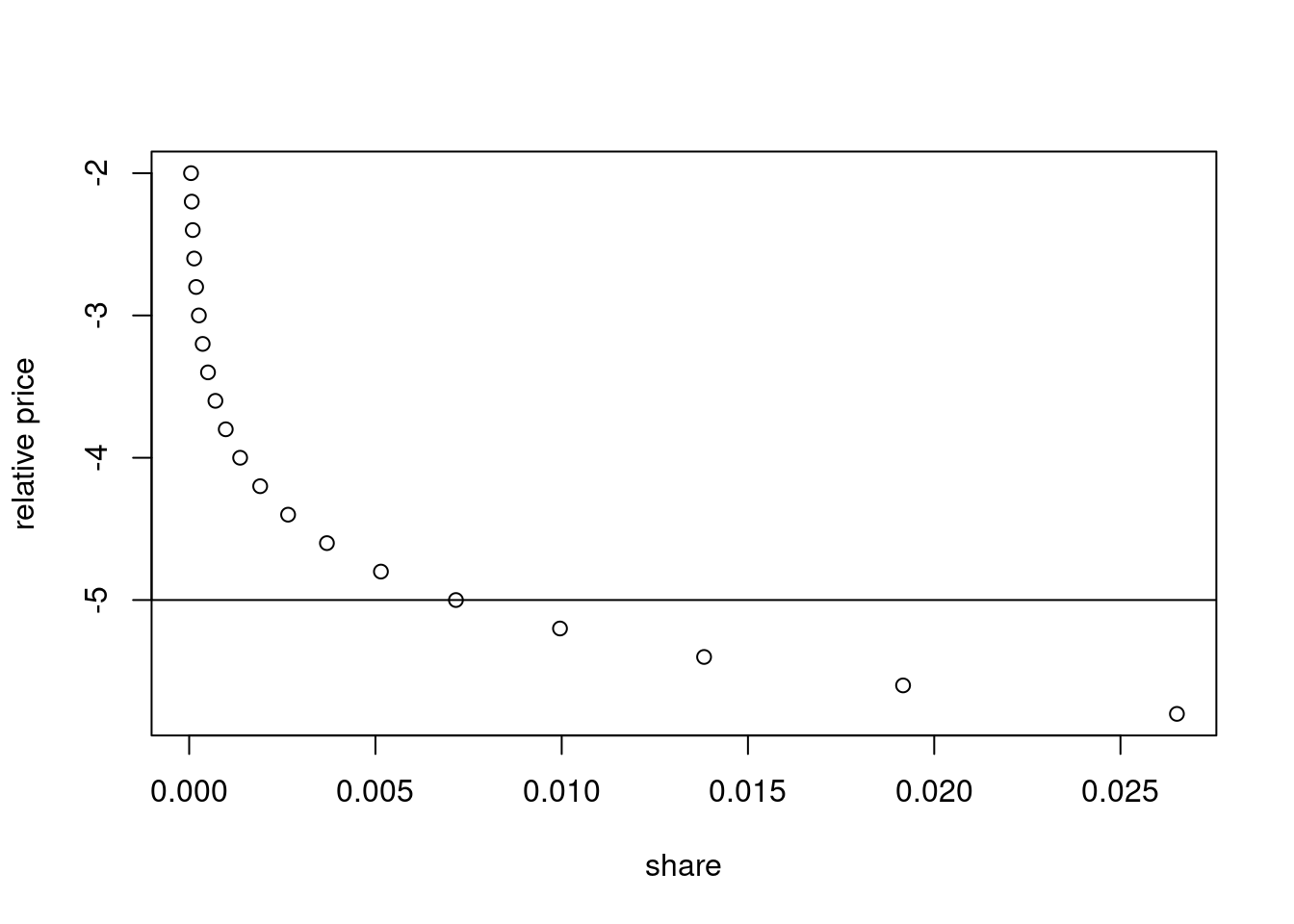
The Figure 3 presents the demand curve for a family size box of Apple Cinnamon Cheerios.

Value of Apple Cinnamon Cheerios

To determine the value of Apple Cinnamon Cheerios family size box we can calculate the area under the demand curve (Hausman 1997).
If we approximate the area with a triangle, we get an annual contribution to consumer welfare of around $271,800 per year for all Dominick’s customers in Chicagoland.⁶ Assuming that Dominick’s had a market share of 25% and that Chicagoland accounts for about $\frac{1}{32}$ of the US population, then this scales to $35m a year. This estimate is substantially lower than Hausman’s estimate of over $60m annually for the United States. Of course, I’m unwilling to argue that my estimate is better with either Bresnahan or Hausman.

(0.5*(-3-acc_demand[5,1])*acc_demand[5,2]*267888011*(52/367))

[1] 271798.6

Discussion and Further Reading

My field, industrial organization, is dominated by what is called structural econometrics. That is, using game theory to estimate the parameters of the model, then using the parameter estimates to make policy predictions. Industrial organization economists believe that these ideas should be used more broadly across economics.

The chapter reconsiders the problem of demand estimation. It allows that prices are determined endogenously in the model. The chapter assumes that prices are actually the result of a game played between rival firms that sell similar products. It shows that we can use a standard IV estimator to estimate the slope of the supply function, then we can use the Nash equilibrium to determine the slope of demand.

It has become standard practice in empirical industrial organization to split the estimation problem in to these two steps. The first step involves standard statistical techniques, while the second step relies on the equilibrium assumptions to back out the policy parameters of interest. Chapter 9 uses this idea to estimate the parameters of interest from auction data (Guerre, Perrigne, and Vuong 2000).

S. Berry, Levinsohn, and Pakes (1995) is perhaps the most important paper in empirical industrial organization. It presents three important ideas. It presents the idea discussed above that logit demand can be inverted which allows for use of the standard instrumental variables approach. This idea is combined with an assumption that prices are determined via equilibrium of a Nash pricing game allowing the parameters of interest to be identified. If this wasn’t enough, it adds the idea of using a flexible model called a mixed logit. All this in one paper used to estimate the demand for cars! However, without Nevo (2000) few would have understood the contributions of S. Berry, Levinsohn, and Pakes (1995). More recently S. T. Berry, Gandhi, and Haile (2013) dug into the assumptions of S. Berry, Levinsohn, and Pakes (1995) to help us understand which are important for identification and which simply simplify the model. MacKay and Miller (2019) have an excellent exposition of the various assumptions needed to estimate demand. What if firms are colluding? Fabinger and Weyl (2013) and Jaffe and Weyl (2013) are good starting places for thinking about estimating demand in that case.

References

Berry, Steven. 1994. “Estimating Discrete-Choice Models of Product Differentiation.” RAND Journal of Economics 25 (2): 242–62.

Berry, Steven T., Amit Gandhi, and Philip A. Haile. 2013. “Connected Substitutes and Invertibility of Demand.” Econometrica 81: 2087–2111.

Berry, Steven, James Levinsohn, and Ariel Pakes. 1995. “Automobile Prices in Market Equilibrium.” Econometrica 60 (4): 889–917.

Bresnahan, Tim. 1997. “The Apple-Cinnamon Cheerios war: valuing new goods, identifying market power, and economic measurement.”

Fabinger, Michal, and Glen Weyl. 2013. “Pass-Through as an Economic Tool: Principle of Incidence Under Imperfect Competition.” Journal of Political Economy 121 (3): 528–83.

Guerre, Emmanuel, Isabelle Perrigne, and Quang Vuong. 2000. “Optimal Nonparametric Estimation of First-Price Auctions.” Econometrica 68 (3): 525–74.

Hausman, Jerry. 1997. “The Economics of New Goods.” In, edited by Timothy Bresnahan and Robert J. Gordon. NBER Studies in Income and Wealth Number 58. The University of Chicago Press.

Hotelling, Harold. 1929. “Stability in Competition.” The Economic Journal 39 (153): 41–57.

Jaffe, Sonia, and Glen Weyl. 2013. “The First-Order Approach to Merger Analysis.” American Economic Journal: Microeconomics 5 (4): 188–218.

MacKay, Alexander, and Nathan Miller. 2019. “Estimating Models of Supply and Demand: Instruments and Covariance Restrictions.”

Nevo, Aviv. 2000. “A Practioner’s Guide to Estimation of Random-Coefficients Logit Models of Demand.” Journal of Economics and Management Strategy 9 (4): 513–48.

Footnotes

1. The next chapter explores this approach.

2. See Chapter 3 for discussion of the assumptions.

3. https://perso.telecom-paristech.fr/eagan/class/igr204/datasets

4. Note in the Berry model we take the log of shares. Remember that log of 0 is infinity, so the code adds a small number to all the shares.

5. The cleaned data is available here: https://sites.google.com/view/microeconometricswithr/

6. The number $267,888,011 is total revenue from the original Dominicks sales data, wcer.csv. Here we used a fraction of the original data (52/367) to get the annual amount.