4.2 The Weighted Quantile Sum (WQS) and its extensions
Taking one step further, researchers might be interested in taking into account the relationship between the exposures and the outcome while summarizing the complex exposure to the mixture of interest. The weighted quantile sum (WQS), developed specifically for the context of environmental mixtures analysis, is an increasingly common approach that allows evaluating a mixture-outcome association by creating a summary score of the mixture in a supervised fashion (Czarnota, Gennings, and Wheeler (2015)), (Carrico et al. (2015)). Specifically, WQS is a statistical model for multivariate regression in high-dimensional dataset that operates in a supervised framework, creating a single score (the weighted quantile sum) that summarizes the overall exposure to the mixture, and by including this score in a regression model to evaluate the overall effect of the mixture on the outcome of interest. The score is calculated as a weighted sum (so that exposures with weaker effects on the outcome have lower weight in the index) of all exposures categorized into quartiles, or more groups, so that extreme values have less impact on the weight estimation.
4.2.1 Model definition and estimation
A WQS regression model takes the following form:
\[g(\mu) = \beta_0 + \beta_1\Bigg(\sum_{i=1}^{c}w_iq_i\Bigg) + \boldsymbol{z'\varphi}\]
The \(\sum_{i=1}^{c}w_iq_i\) term represents the index that weights and sums the components included in the mixture. As such, \(\beta_1\) will be the parameter summarizing the overall effect to the (weighted) mixture. In addition, the model will also provide an estimate of the individual weights \(w_i\) that indicate the relative importance of each exposure in the mixture-outcome association.
To estimate the model, the data may be split in a training and a validation dataset: the first one to be used for the weights estimation, the second one to test for the significance of the final WQS index. The weights are estimated through a bootstrap and constrained to sum to one and to be bounded between zero and one: \(\sum_{i=1}^{c}w_i=1\) and \(0 \leq w_i \leq 1\). For each bootstrap sample (usually \(B=100\) total samples) a dataset is created sampling with replacement from the training dataset and the parameters of the model are estimated through an optimization algorithm.
Once the weights are estimated, the model is fitted in order to find the regression coefficients in each ensemble step. After the bootstrap ensemble is completed, the estimated weights are averaged across bootstrap samples to obtain the WQS index:
\[WQS = \sum_{i=1}^c \bar{w}_iq_i\]
Typically weights are estimated in a training set then used to construct a WQS index in a validation set, which can be used to test for the association between the mixture and the health outcome in a standard generalized linear model, as:
\[g(\mu) = \beta_0 + \beta_1WQS + \boldsymbol{z'\varphi}\]
After the final model is complete one can test the significance of the \(\beta_1\) to see if there is an association between the WQS index and the outcome. In the case the coefficient is significantly different from 0 then we can interpret the weights: the highest values identify the associated components as the relevant contributors in the association. A selection threshold can be decided a priori to identify those chemicals that have a significant weight in the index.
4.2.2 The unidirectionality assumption
WQS makes an important assumption of uni-direction (either a positive or a negative) of all exposures with respect to the outcome. The model is inherently one-directional, in that it tests only for mixture effects positively or negatively associated with a given outcome. In practice analyses should therefore be run twice to test for associations in either direction.
The one-directional index allows not to incur in the reversal paradox when we have highly correlated variables thus improving the identification of bad actors.
4.2.3 Extensions of the original WQS regression
- Dependent variables
The WQS regression can be generalized and applied to multiple types of dependent variables. In particular, WQS regression has been adapted to four different cases: logistic, multinomial, Poisson and negative binomial regression. For these last two cases it is also possible to fit zero-inflated models keeping the same objective function used to estimate the weights as for the Poisson and negative binomial regression but taking into account the zero inflation fitting the final model.
- Random selection
A novel implementation of WQS regression for high-dimensional mixtures with highly correlated components was proposed in Curtin et al. (2021). This approach applies a random selection of a subset of the variables included in the mixture instead of the bootstrapping for parameter estimation. Through this method we are able to generate a more de-correlated subsets of variables and reduce the variance of the parameter estimates compared to a single analysis. This extension was shown to be more effective compared to WQS in modeling contexts with large predictor sets, complex correlation structures, or where the numbers of predictors exceeds the number of subjects.
- Repeated holdout validation for WQS regression
One limit of WQS is the reduced statistical power caused by the necessity to split the dataset in training and validation sets. This partition can also lead to unrepresentative sets of data and unstable parameter estimates. A recent work from Tanner, Bornehag, and Gennings (2019) showed that conducing a WQS on the full dataset without splitting in training and validation produces optimistic results and proposed to apply a repeated holdout validation combining cross-validation and bootstrap resampling. They suggested to repeatedly split the data 100 times with replacement and fit a WQS regression on each partitioned dataset. Through this procedure we obtain an approximately normal distribution of the weights and the regression parameters and we can apply the mean or the median to estimate the final parameters. A limit of this approach is the higher computational intensity.
- Penalized weights and 2 indexes
The most recent extension of WQS to date, presented in Renzetti, Gennings, and Calza (2023), allows simultaneous estimation of the positive and negative index. This is implemented in the R package and improves the accuracy of the parameter estimates when considering a mixture of elements that can have both a protective and a harmful effect on the outcome.
- Other extensions
To complete the set of currently available extensions of this approach, it is finally worthy to mention the Bayesian WQS (Colicino et al. (2020)), which also allows relaxing the uni-directional assumption, and the lagged WQS (Gennings et al. (2020)), which deals with time-varying mixtures of exposures to understand the role of exposure timing.
4.2.4 Quantile G-computation
Quantile G-computation was introduced by Keil et al. (2020) as a potential approach to overcome the main limitations of WQS (uni-directional assumption) while also improving the causal interpretation of the results Quantile g-Computation estimates the overall mixture effect with the same procedure used by WQS, but estimating the parameters of a marginal structural model, rather than a standard regression. In this way, under common assumptions in causal inference such as exchangeability, causal consistency, positivity, no interference, and correct model specification, this model will also improve the causal interpretation of the overall effect. Importantly, the flexibility of marginal structural models also allows incorporating non-linearities in the contribution of each exposure to the score. The introduction to R code for this approach, included in the previous version of this online material, has been removed since the online documentation for implementing qgcomp has substantially improved. In particular, the reader can refer to this link.
As a note of caution, it is important to note that by removing the assumption of uni-directionality, quantile G-computations is subject to severe limitations in the presence of high levels of correlations. Here for example, results from fitting the model on our set of simulated data, showing a strikingly high (and, as we know since data are simulated, wrong) negative weight for \(X_3\).
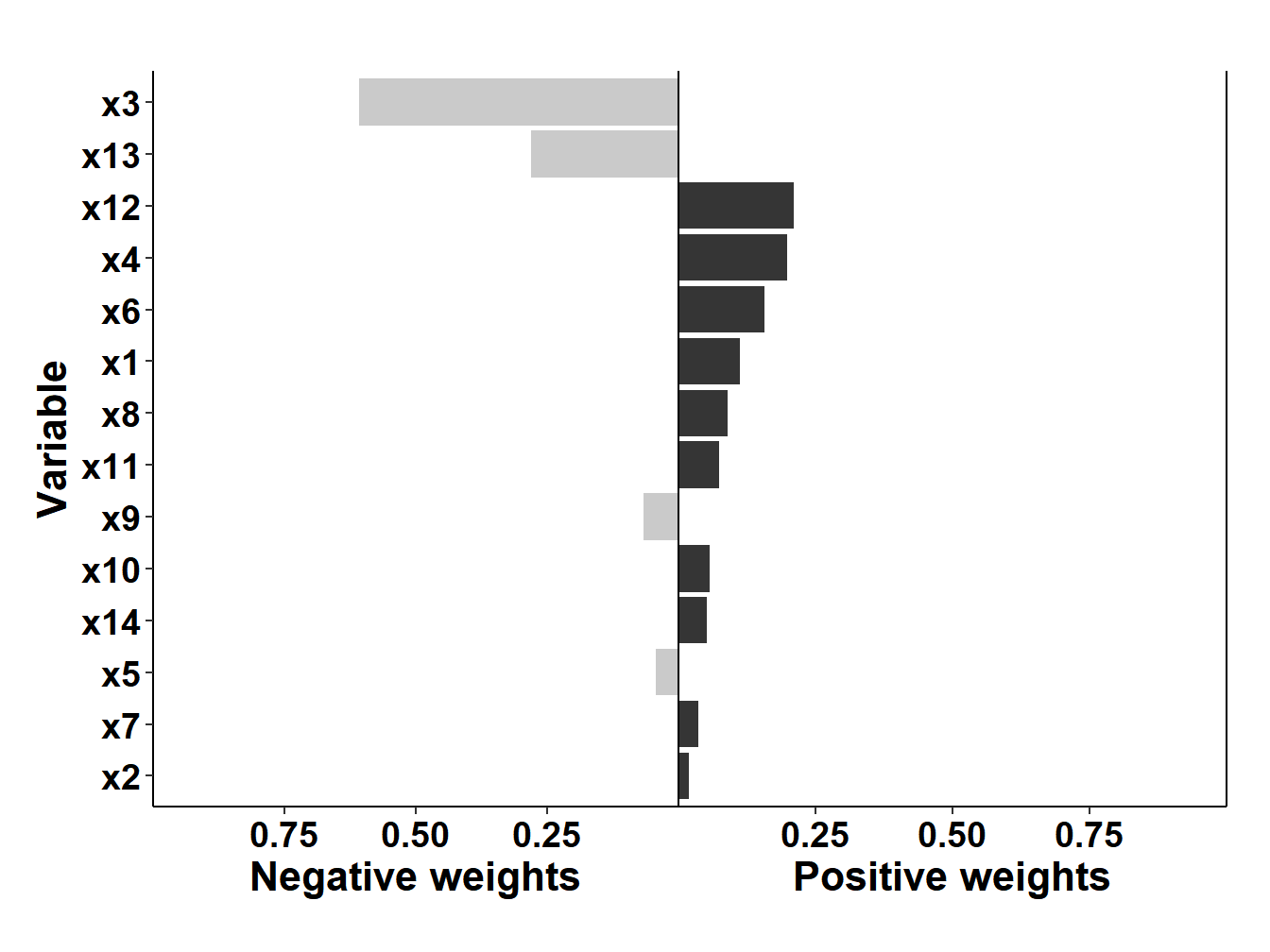
Figure 4.1: qGcomp results on simulated data
4.2.5 WQS regression in R
WQS is available in the R package gWQS (standing for generalized WQS). Documentation and guidelines can be found here.
[Note that the vignette and package have been updated as on November 2023. Please refer to the above link rather than on the code reported here (last updated in December 2021)]
Fitting WQS in R will require some additional data management. First of all, both gWQS and qgcomp will require an object with the names of the exposures, rather than a matrix with the exposures themselves.
exposure<- names(data2[,3:16])The following lines will fit a WQS regression model for the positive direction, with a 40-60 training validation split, and without adjusting for covariates. The reader can refer to the link above for details on all available options.
results1 <- gwqs(y ~ wqs, mix_name = exposure, data = data2, q = 4,
                 validation = 0.6, b = 10, b1_pos = T, b1_constr = F,
                 family = "gaussian", seed = 123)
After fitting the model, this line will produce a barplot with the weights as well as the summary of results (overall effect and weights estimation), presented in Table 4.1 and Figure 4.1/
gwqs_barplot(results1, tau=NULL)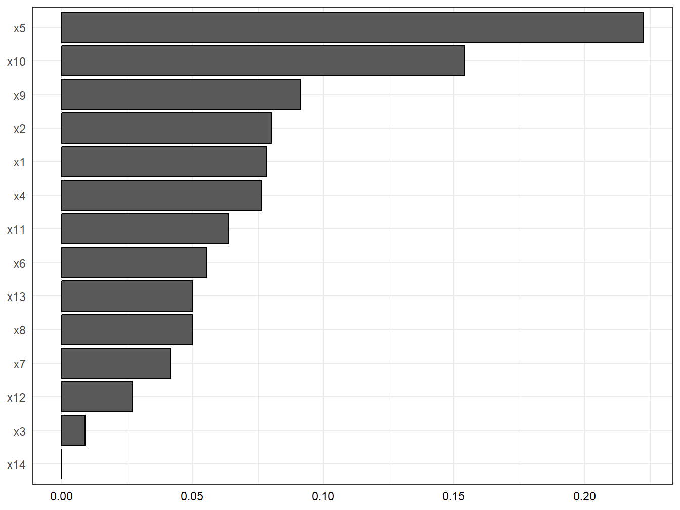
Figure 4.2: WQS: weights estimation in the simulated dataset
| mix_name | mean_weight | |
|---|---|---|
| x5 | x5 | 0.2223475 |
| x10 | x10 | 0.1541689 |
| x9 | x9 | 0.0912947 |
| x2 | x2 | 0.0801335 |
| x1 | x1 | 0.0784043 |
| x4 | x4 | 0.0764677 |
| x11 | x11 | 0.0638050 |
| x6 | x6 | 0.0556224 |
| x13 | x13 | 0.0502334 |
| x8 | x8 | 0.0499036 |
| x7 | x7 | 0.0416033 |
| x12 | x12 | 0.0270018 |
| x3 | x3 | 0.0090138 |
| x14 | x14 | 0.0000000 |
To estimate the negative index, still without direct constraint on the actual \(\beta\), we change the b1_pos option to FALSE. In this situation, all bootstrap samples provide a positive coefficient. This suggests that we are in a situation where all covariates have a positive (or null) effect. Even constraining the coefficient would likely not make any difference in this case - coefficients would either be all around 0, or the model will not converge.
To adjust the positive WQS regression model for confounders we can add them in the model as presented here:
results1_0_adj <- gwqs(y ~ wqs+z1+z2+z3, mix_name = exposure, data = data2,
                       q = 4, validation = 0.6, b = 10, b1_pos = T,
b1_constr = F, family = "gaussian", seed = 123)gwqs_barplot(results1_0_adj, tau=NULL)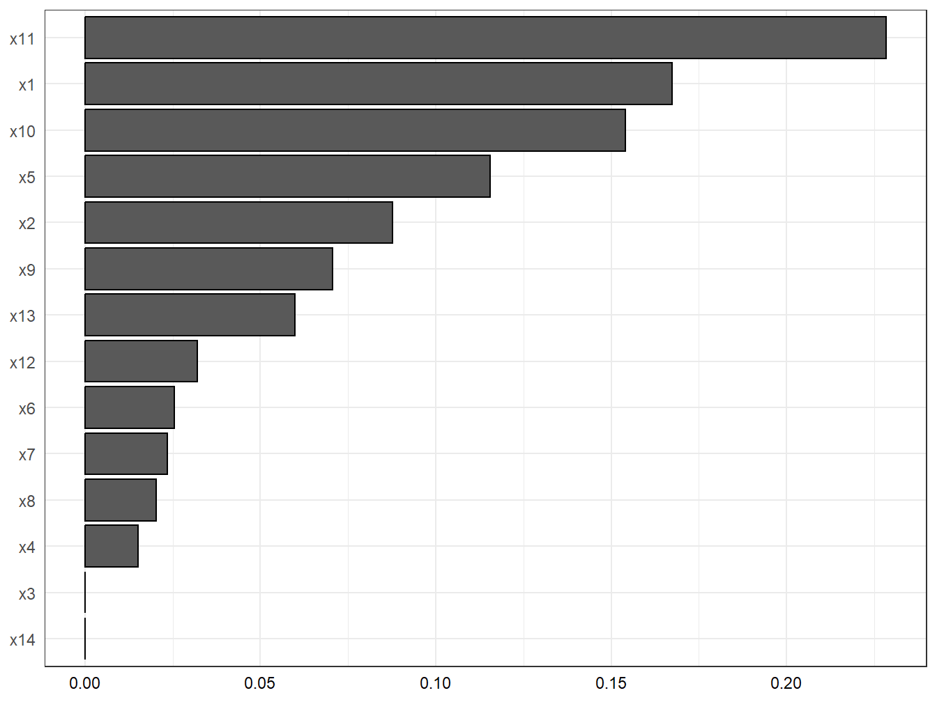
Figure 4.3: WQS: weights estimation with covariates adjustment in the simulated dataset
After adjustment the association is largely attenuated, and the weights of the most important contributors change both in magnitude as well as in ranking (Figure 4.2). This implies that the three confounders have a different effect on each of the components (e.g. the contribution of \(X_6\) was attenuated before adjusting, while the contribution of \(X_4\) was overestimated).
4.2.6 Example from the literature
Thanks for its easy implementation in statistical software and the development of the several discussed extensions, WQS is rapidly becoming one of the most common techniques used by investigators to evaluate environmental mixtures.
As an illustrative example on how methods and results can be presented the reader can refer to a paper from Deyssenroth et al. (2018), evaluating the association between 16 trace metals, measured in post-partum maternal toe nails in about 200 pregnant women from the Rhode Island Child Health Study, and small for gestational age (SGA) status. Before fitting WQS the Authors conduct a preliminary analysis using conditional logistic regression, which indicates that effects seem to operate in both directions (Figure 4.5).
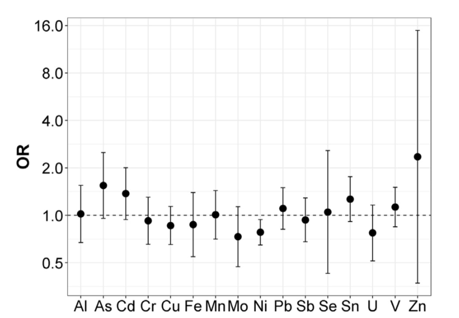
Figure 4.4: Conditional logistic regression results from Deyssenroth et al. 2018
As a consequence, WQS results are presented for both the positive and negative directions, summarizing both weights estimates and total effects in a clear and informative figure (Figure 4.6).
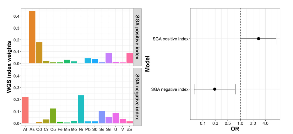
Figure 4.5: WQS results from Deyssenroth et al. 2018