3.2 Penalized regression approaches
An important set of models that can be very useful in the context of environmental mixtures are penalized regression approaches. These methods are directly built as extensions of standard OLS by incorporating a penalty in the loss function (hence the name). Their popularity in environmental epidemiology is due to the fact that this penalization procedure tends to decrease the influence of collinearity by targeting the overall variability of the model, thus improving the performance of the regression in the presence of high levels of correlations between included covariates. As always, however, everything comes for a price, and the improvement in the variance is achieved by introducing some bias (specifically, coefficients will be shrunk towards zero, reason why these approaches are also referred to as shrinkage procedures).
3.2.1 Bias-variance tradeoff
The word bias usually triggers epidemiologists’ antennas, so it is important to understand what we mean by “introducing some bias” and how this can be beneficial in our context. To do so, let’s begin by refreshing the basic math behind the estimation of a classical multiple regression. In linear regression modeling, we aim at predicting \(n\) observations of the response variable, \(Y\), with a linear combination of \(m\) predictor variables, \(X\), and a normally distributed error term with variance \(\sigma^2\): \[Y=X\beta+\epsilon\] \[\epsilon\sim N(0, \sigma^2)\]
We need a rule to estimate the parameters, \(\beta\), from the sample, and a standard choice to do so is by using ordinary least square (OLS), which produce estimates \(\hat{\beta}\) by minimizing the sum of squares of residuals is as small as possible. In other words, we minimize the following loss function:
\[L_{OLS}(\hat{\beta})=\sum_{i=1}^n(y_i-x_i'\hat{\beta})^2=\|y-X\hat{\beta}\|^2\]
Using matrix notation, the estimate turns out to be :
\[\hat{\beta}_{OLS}=(X'X)^{-1}(X'Y)\]
To evaluate the performance of an estimator, there are two critical characteristics to be considered: its bias and its variance. The bias of an estimator measures the accuracy of the estimates:
\[Bias(\hat{\beta}_{OLS})=E(\hat{\beta}_{OLS})-\beta\]
The variance, on the other hand, measures the uncertainty of the estimates:
\[Var(\hat{\beta}_{OLS})=\sigma^2(X'X)^{-1}\]
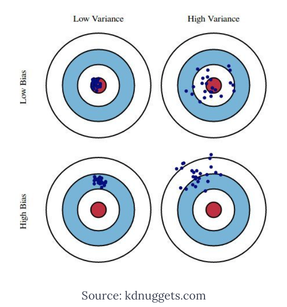
Figure 3.6: Archery example
Think of the estimator as an olympic archer (Figure 3.6). The best performer will be an archer with low bias and low variance (top-left), who consistently aims the target for every estimate. An archer with low bias but high variance will be the one who will shoot inconsistently around the center (top-right), but we may also have an archer with high bias and low variance, who is extremely precise in consistently shooting at the wrong target (bottom-left). Now, the OLS estimator is an archer who is designed to be unbiased, but in certain situations might have a very high variance, situation that commonly happens when collinearity is a threat, as documented by the inflation in the variance calculated by the VIF.
To assess the overall performance an estimator by taking into account both bias and variance, one can look at the Mean Squared Error (MSE), defined as the sum of Variance and squared Bias.
\[MSE=\frac{1}{n}\sum_{i=1}^n(Y_i-\hat{Y_i})^2=Var(\hat{\beta})+Bias^2(\hat{\beta})\]
The basic idea of bias-variance trade-off is to introduce some bias in order to minimize the mean squared error in those situation where the performances of OLS are affected by high variance. This is achieved by augmenting the loss function by introducing a penalty. While there are several ways of achieving this, we will here focus on three common penalty functions that originate Ridge, LASSO, and Elastic-Net regression, with the latter being a generalized version of the previous two.
3.2.2 Ridge regression
Ridge regression augments the OLS loss function as to not only minimize the sum of squared residuals, but also penalize the size of the parameter estimates, shrinking them towards zero
\[L_{ridge}(\hat{\beta})=\sum_{i=1}^n(y_i-x_i'\hat{\beta})^2+\lambda\sum_{j=1}^m\hat{\beta}_j^2=\|y-X\hat{\beta}\|^2+\lambda\|\hat{\beta}\|^2\]
Minimizing this equation provides this solution for the parameters estimation: \[\hat{\beta}_{ridge}=(X'X+\lambda I)^{-1}(X'Y)\] where \(\lambda\) is the penalty and \(I\) an identity matrix
We can notice that as \(\lambda\rightarrow 0\), \(\hat{\beta}_{ridge}\rightarrow\hat{\beta}_{OLS}\), while as \(\lambda\rightarrow \infty\), \(\hat{\beta}_{ridge}\rightarrow 0\). In words, setting \(\lambda\) to 0 is like using OLS, while the larger its value, the stronger the penalization. The unique feature of Ridge regression, as compared to other penalization techniques, is that coefficients can be shrunk over and over but will never reach 0. In other words, all covariates will always remain in the model, and Ridge does not provide any form of variable selection.
It can be shown that as \(\lambda\) becomes larger, the variance decreases and the bias increases. How much are we willing to trade? There are several approaches that can be used to choose for the best value of \(\lambda\):
- Choose the \(\lambda\) that minimizes the MSE
- Use a traditional approach based on AIC or BIC criteria, to evaluate the performance of the model in fitting the data. While software tend to do the calculation automatically, it is important to remember that the degrees of freedom of a penalized model, needed to calculate such indexes, are different from the degrees of freedom of a OLS model with the same number of covariates/individuals
- Finally, a recommended procedure is based on cross-validation, focusing more on the predictive performances of the model. More specifically, to avoid the the model perfectly fits our data with poor generalizability (situation commonly known as overfitting in the machine learning vocabulary), we tend to select the model corresponding to the largest \(\lambda\) within one unit of standard deviation around the \(\lambda\) that minimizes the MSE
Let’s turn to our illustrative example to see Ridge regression in practice. Given that both ridge and lasso are special cases of elastic net, we are going to use the glmnet package for all three approaches. Alternative approaches are available and could be considered. First we should define a set of potential values of \(\lambda\) that we will then evaluate (lambdas_to_try). To select the optimal \(\lambda\) we are then going to use the 10-fold cross validation approach, which can be conducted with the cv.glmnet command. Note that with option standardize=TRUE exposure will be standardized; this can be set to FALSE if standardization has been already conducted. Also, the option alpha=0 has to be chosen to conduct Ridge regression (we will see later that Ridge is an Elastic Net model where an \(\alpha\) parameter is equal to 0).
ridge_cv <- cv.glmnet(X, Y, alpha = 0, lambda = lambdas_to_try,
                      standardize = TRUE, nfolds = 1000)
We can now plot the MSE at different levels of \(\lambda\). While the goal is to find the model that minimizes the MSE (lambda.min), we don’t want the model to overfit our data. For this reason we tend to select the model corresponding to the largest \(\lambda\) within one unit of standard deviation around lambda.min (lambda.1se). Figure 3.7 shows the plot of MSE over levels of \(\lambda\), also indicating these two values of interest (the vertical dashed lines).
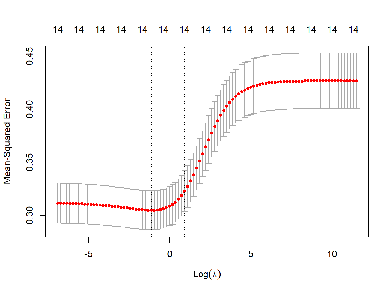
Figure 3.7: MSE vs lambda for ridge regression in simulated data
# lowest lambda
lambda_cv_min <- ridge_cv$lambda.min
lambda_cv_min
## [1] 0.3199267# Best cross-validated lambda
lambda_cv <- ridge_cv$lambda.1se
lambda_cv## [1] 2.477076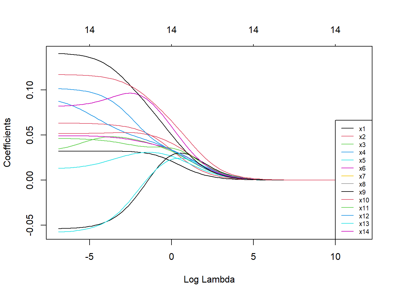
Figure 3.8: Coefficients trajectories for ridge regression in simulated dataset
The starting values on the left of the figure are the ones from OLS estimation, and then we see how coefficients get shrunk at increasingly higher levels of \(\lambda\). Note that the shrinkage is operated on the entire model, and for this reason individual trajectories are not necessarily forced to decrease (here some coefficients become larger before getting shrunk). Also, from the numbers plotted on top of the figure, indicating the number of coefficients that are still included in the model, we can see that coefficients only tend asymptotically to 0 but are never really removed from the model.
Finally, we can summarize the results of our final model for the selected value of lambda:
model_cv <- glmnet(X, Y, alpha = 0, lambda = lambda_cv, standardize = TRUE)| Estimate | |
|---|---|
| x1 | 0.013 |
| x2 | 0.021 |
| x3 | 0.024 |
| x4 | 0.024 |
| x5 | 0.020 |
| x6 | 0.026 |
| x7 | 0.029 |
| x8 | 0.031 |
| x9 | 0.030 |
| x10 | 0.026 |
| x11 | 0.024 |
| x12 | 0.038 |
| x13 | 0.031 |
| x14 | 0.047 |
These results, presented in Table 3.4, can provide some useful information but are of little use in our context. For example, we know from our VIF analysis that the coefficients for \(X_{12}\) and \(X_{13}\) are affected by high collinearity, but we would like to understand whether a real association exists for both exposures or whether one of the 2 is driving the cluster. To do so, we might prefer to operate some sort of variable selection, constructing a penalty so that non-influential covariates can be set to 0 (and therefore removed). This is what LASSO does.
3.2.3 LASSO
Lasso, standing for Least Absolute Shrinkage and Selection Operator, also adds a penalty to the loss function of OLS. However, instead of adding a penalty that penalizes sum of squared residuals (L2 penalty), Lasso penalizes the sum of their absolute values (L1 penalty). As a results, for high values of \(\lambda\), many coefficients are exactly zeroed under lasso, which is never the case in ridge regression (where 0s are the extreme case as \(\lambda\rightarrow\infty\)). Specifically, the Lasso estimator can be written as
\[L_{lasso}(\hat{\beta})=\sum_{i=1}^n(y_i-x_i'\hat{\beta})^2+\lambda\sum_{j=1}^m|\hat{\beta}_j|\]
As before, let’s turn to our illustrative example to understand properties and interpretation. The procedure in R is exactly the same, with the only difference that the parameter \(\alpha\) is set to 1. First, let’s identify the optimal value of \(\lambda\) using the cross validation procedure (Figure 3.9),
lasso_cv <- cv.glmnet(X, Y, alpha = 1, lambda = lambdas_to_try,
                      standardize = TRUE, nfolds = 1000)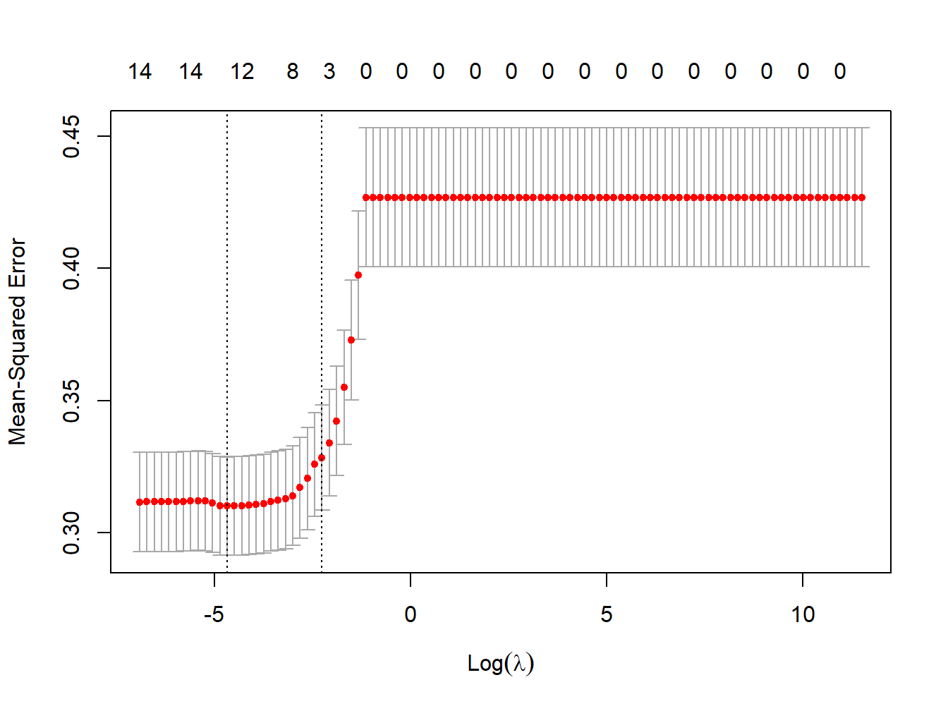
Figure 3.9: MSE vs lambda for lasso regression in the simulated dataset
# lowest lambda
lambda_cv_min_lasso <- lasso_cv$lambda.min
lambda_cv_min_lasso
## [1] 0.009326033# Best cross-validated lambda
lambda_cv_lasso <- lasso_cv$lambda.1se
lambda_cv_lasso## [1] 0.1047616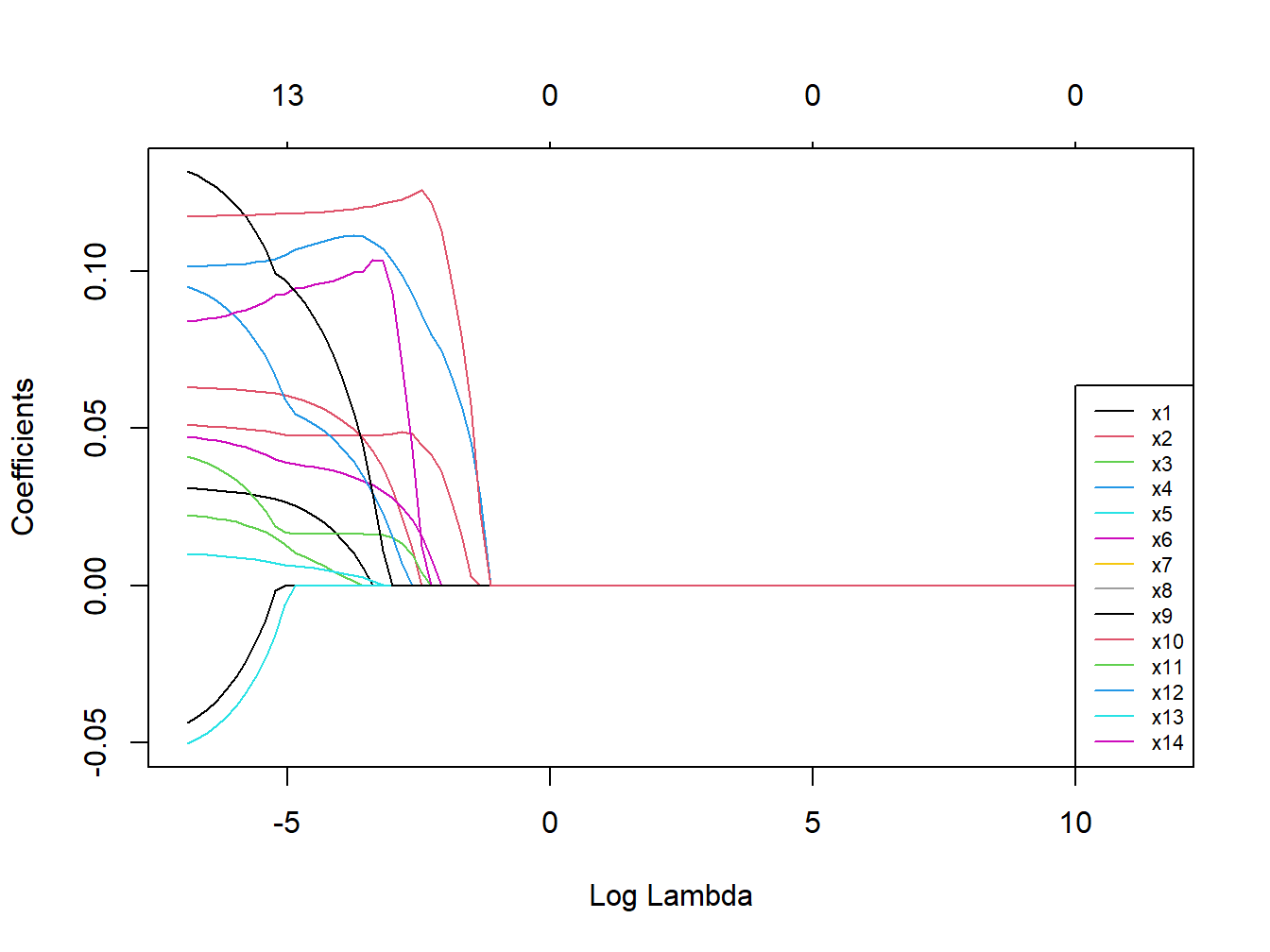
Figure 3.10: Coefficients trajectories for lasso regression in the simulated dataset
We see that, differently from what observed in Ridge regression, coefficients are shrunk to a point where they exactly equal 0, and are therefore excluded from the model. The numbers on top of Figure 3.9 show how many exposures are left in the model at higher levels of \(\lambda\). Finally, let’s take a look at the results of the optimal selected model, presented in Table 3.5.
model_cv_lasso <- glmnet(X, Y, alpha = 1, lambda = lambda_cv_lasso,
standardize = TRUE)| Estimate | |
|---|---|
| x1 | 0.000 |
| x2 | 0.000 |
| x3 | 0.000 |
| x4 | 0.080 |
| x5 | 0.000 |
| x6 | 0.009 |
| x7 | 0.000 |
| x8 | 0.041 |
| x9 | 0.000 |
| x10 | 0.000 |
| x11 | 0.000 |
| x12 | 0.000 |
| x13 | 0.000 |
| x14 | 0.122 |
The final model selects only 4 covariates, while all other drop to 0. If we look at our two established groups of correlated exposures, \(X_4\) and \(X_{12}\) are selected, while the others are left out.
In general, Lasso’s results may be very sensitive to weak associations, dropping coefficients that are not actually 0. Lasso can set some coefficients to zero, thus performing variable selection, while ridge regression cannot. The two methods solve multicollinearity differently: in ridge regression, the coefficients of correlated predictors are similar, while in lasso, one of the correlated predictors has a larger coefficient, while the rest are (nearly) zeroed. Lasso tends to do well if there are a small number of significant parameters and the others are close to zero (that is - when only a few predictors actually influence the response). Ridge works well if there are many large parameters of about the same value (that is - when most predictors impact the response).
3.2.4 Elastic net
Rather than debating which model is better, we can directly use Elastic Net, which has been designed as a compromise between Lasso and Ridge, attempting to overcome their limitations and performing variable selection in a less rigid way than Lasso. Elastic Net combines the penalties of ridge regression and Lasso, aiming at minimizing the following loss function
\[L_{enet}(\hat{\beta})=\frac{\sum_{i=1}^n(y_i-x_i'\hat{\beta})^2}{2n}+\lambda\left(\frac{1-\alpha}{2}\sum_{j=1}^m\hat{\beta}_j^2+\alpha\sum_{j=1}^m|\hat{\beta}_j|\right)\]
where \(\alpha\) is the mixing parameter between ridge (\(\alpha\)=0) and lasso (\(\alpha\)=1). How this loss function is derived, given the ridge and lasso ones, is described in Zou and Hastie (2005). Procedures to simultaneously tune both \(\alpha\) and \(\lambda\) to retrieve the optimal combinations are available and developed in the R package caret. For simplicity we will here stick on glmnet, which requires pre-defining a value for \(\alpha\). One can of course fit several models and compare them with common indexes such as AIC or BIC. To ensure some variable selection, we may for example choose a value of \(\lambda\) like 0.7, closer to Lasso than to Ridge. Let’s fit an Elastic Net model, with \(\alpha=0.7\) in our example. First, we need to select the optimal value of \(\lambda\) (Figure 3.11).
enet_cv <- cv.glmnet(X, Y, alpha = 0.7, lambda = lambdas_to_try,
                     standardize = TRUE, nfolds = 1000)
Figure 3.11: MSE vs lambda for elastic net regression in the simulated dataset
lambda_cv_min_enet <- enet_cv$lambda.min
lambda_cv_min_enet
## [1] 0.01353048# Best cross-validated lambda
lambda_cv_enet <- enet_cv$lambda.1se
lambda_cv_enet## [1] 0.1261857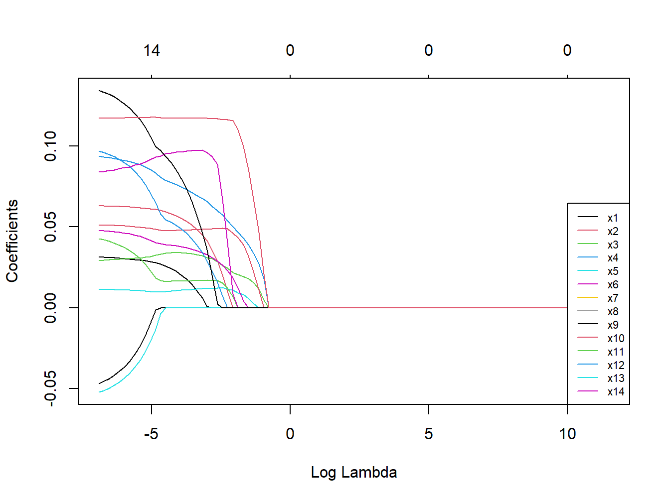
Figure 3.12: Coefficients trajectories for elastic net
We see that coefficients are shrunk to a point where they exactly equal 0, and therefore excluded from the model, but that this happens more conservatively as compared to Lasso (as documented from the numbers on top). Let’s take a look at the results of the optimal selected model (Table 3.6).
model_cv_enet <- glmnet(X, Y, alpha = 0.7, lambda = lambda_cv_enet,
standardize = TRUE)| Estimate | |
|---|---|
| x1 | 0.000 |
| x2 | 0.000 |
| x3 | 0.022 |
| x4 | 0.050 |
| x5 | 0.011 |
| x6 | 0.018 |
| x7 | 0.000 |
| x8 | 0.046 |
| x9 | 0.007 |
| x10 | 0.000 |
| x11 | 0.000 |
| x12 | 0.009 |
| x13 | 0.000 |
| x14 | 0.116 |
As expected, less covariates are dropped to 0. Unfortunately, however, all components of the group of correlated covariates \(X_3-X_5\) remain in the model, and we are not able to identify the key actor of that group. Results, however, seem to agree with multiple regression in indicating \(X_6\) and \(X_{12}\) as the main predictors of the outcome.
Penalized regression techniques allow including confounders, which can be done by specifying them in the model as in a regular OLS model. However, we may want them to be involved in the selection process. To such end, the best way is to include them in the matrix of covariates to be penalized, but inform the CV procedure that you don’t want their coefficients to be modified. The following chunk of code will do that. Note that, regardless of how large \(\lambda\) will be, the three confounders will remain non-penalized in the model, as documented from the numbers on top.
enet_cv_adj <- cv.glmnet(X, Y, alpha = 0.7, lambda = lambdas_to_try,
                     standardize = TRUE, nfolds = 1000,
                     penalty.factor=c(rep(1,ncol(X) - 3),0,0,0))
3.2.5 Additional notes
We have covered the basic theory of penalized regression techniques (also referred to with other common terminology such as shrinkage procedures, or regularization processes). Before moving to the presentation of two applications of these techniques in environmental epidemiology, let’s mention some additional details.
- Replicate results in classical OLS
When Elastic Net is used to describe associations in population-based studies, it is common practice to also present a final linear regression model that only includes those predictors that were selected from the penalized approach. This model will ensure better interpretation of the coefficients, and hopefully not be subject anymore to issues of collinearity that the selection should have addressed.
- Grouped Lasso
In some settings, the predictors belong to pre-defined groups, or we might have observed well-defined subgroups of exposures from our PCA. In this situation one may want to shrink and select together the members of a given group, which can be achieved with grouped Lasso. The next subsection will provide alternative regression approaches where preliminary grouping information can be used to address some limitations of standard regression.
- Time-to-event outcomes
Recent developments allow fitting Elastic Net with time-to-event outcomes, within the context of a regularized Cox regression model. Given the popularity of this method in epidemiology it is reasonable to expect that this approach will become more popular in the context of environmental mixture since (as we will see in next sections) methods that were built ad-hoc do not always account for these types of outcomes. A first R package was develop in 2011 (coxnet), fully documented here, and those algorithms for right-censored data have also been included in the most recent version of glmnet
- Non-linear associations
An implicit assumption we have made so far is that each covariate included in the model has a linear (or log-linear) effect on the outcome of interest. We know that this is often not true (several environmental exposures, for example, have some kind of plateau effect) and we might want to be able to incorporate non-linearities in our analyses. While classical regression can flexibly allow incorporating non-linearities by means of categorical transformations or restricted cubic splines, this is not of straightforward application in penalized regression. In complex settings where strong departures from linearity are observed in preliminary linear regressions, one should probably consider more flexible techniques such as BKMR (Section 5).
3.2.6 Elastic Net and environmental mixtures
Using Elastic Net to evaluate the association between a mixture of environmental exposures and a health outcome is becoming increasingly popular. A nice and rigorous application of the method can be found in Lenters et al. (2016), evaluating co-exposure to 16 chemicals as they relate to birth weight in 1250 infants. Figure 3.13 presents the correlation plot from the manuscript.
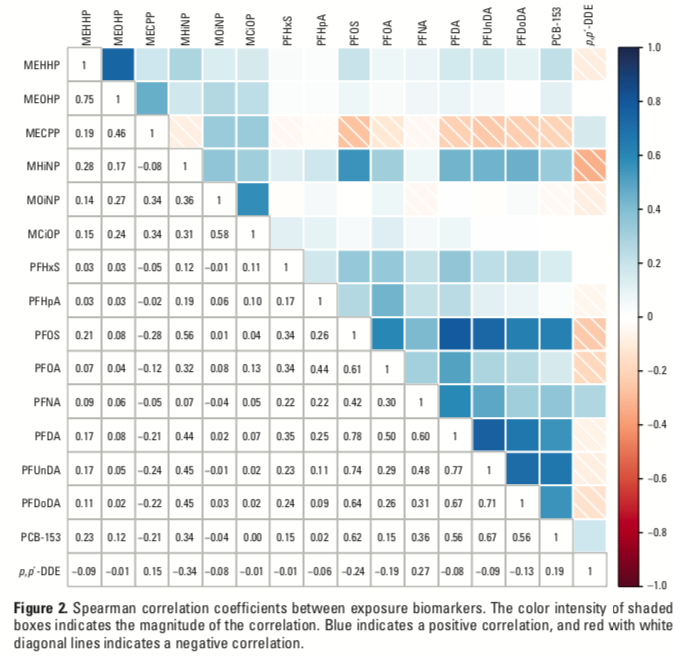
Figure 3.13: Correlation plot from Lenters et al. 2016
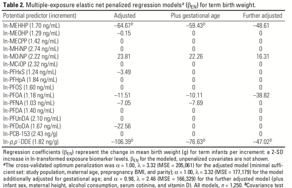
Figure 3.14: Elastic net regression results from Lenters et al. 2016
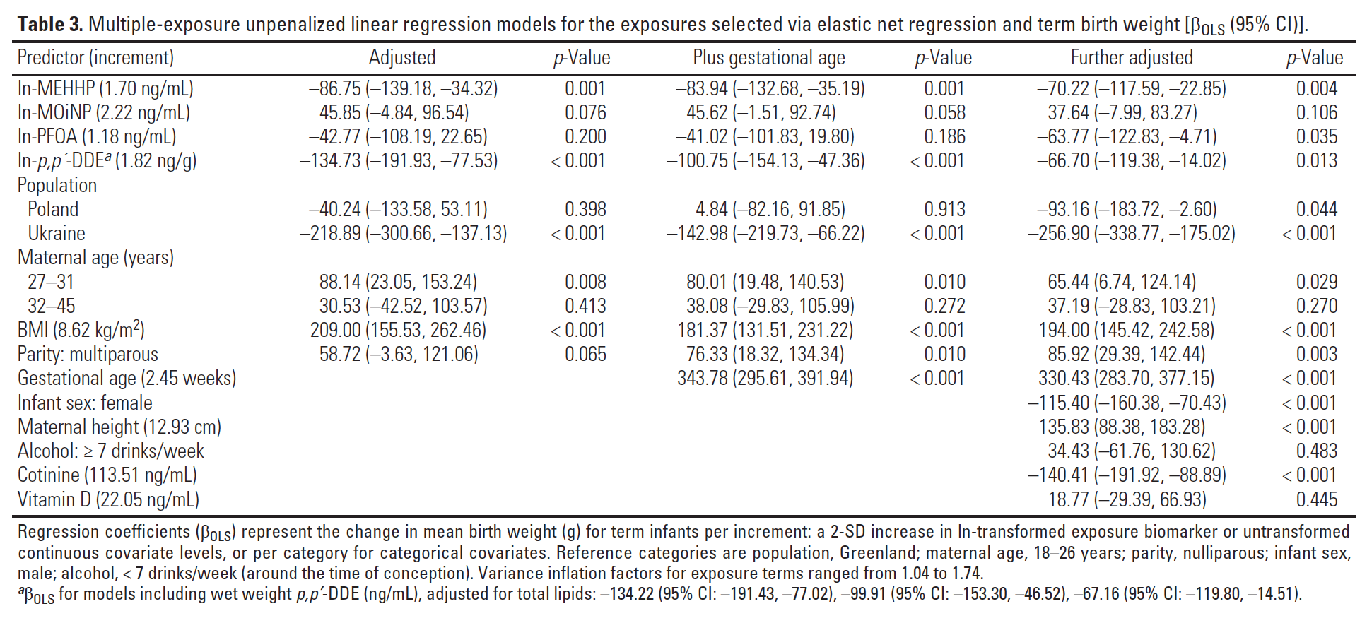
Figure 3.15: Final results from Lenters et al. 2016
Another application that thoroughly reports methods presentation, stating all assumptions and clearly discussing the results, can be found in Vriens et al. (2017), evaluating environmental pollutants and placental mitochondrial DNA content in infants. Figure 3.16 presents the correlation plot reported in the paper.
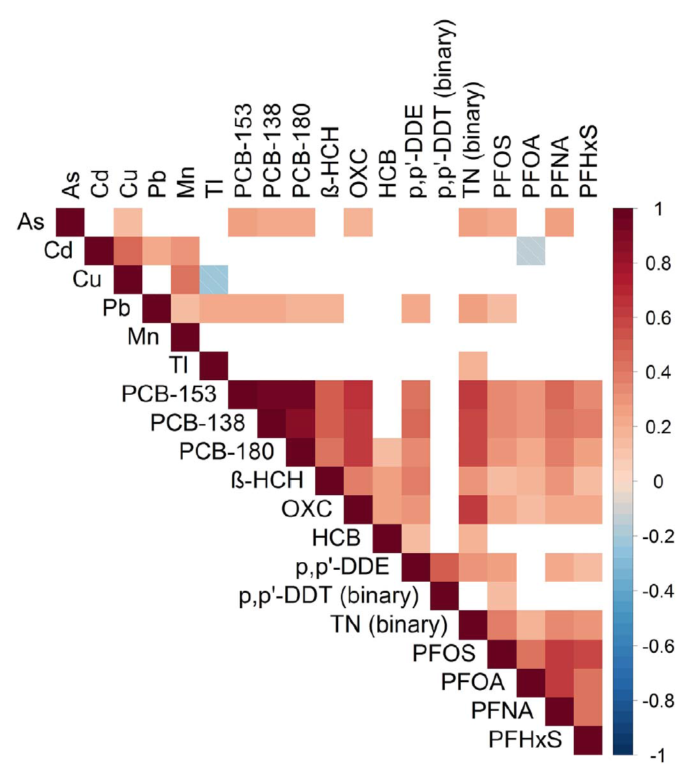
Figure 3.16: Correlation plot from Vriens et al. 2017
Several detailed figures are used to present results providing the reader with all necessary tools to understand associations and provide clear interpretation, and are reported in Figures 3.17 and 3.18.
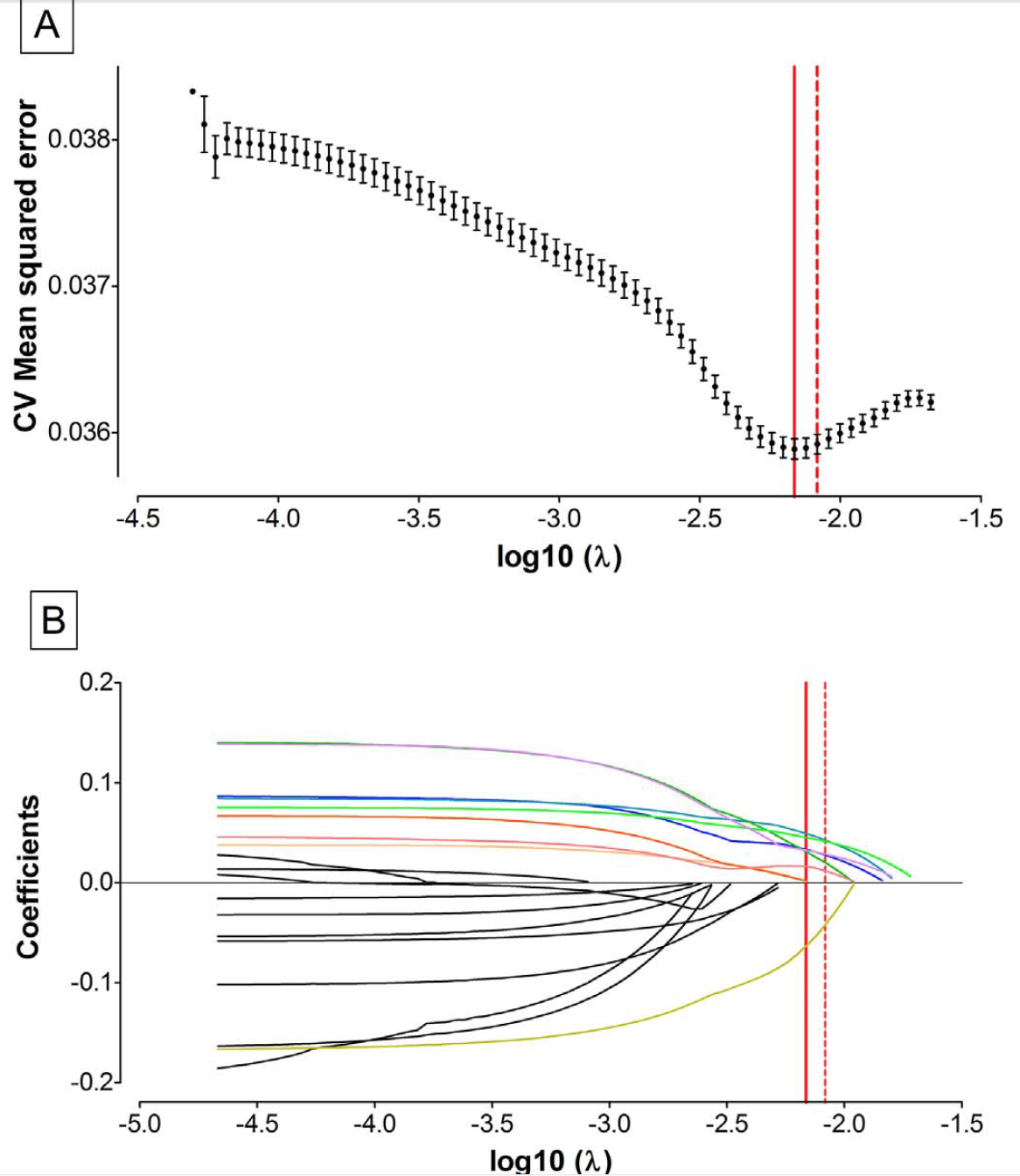
Figure 3.17: MSE and coefficients’ trajectories from Vriens et al. 2017
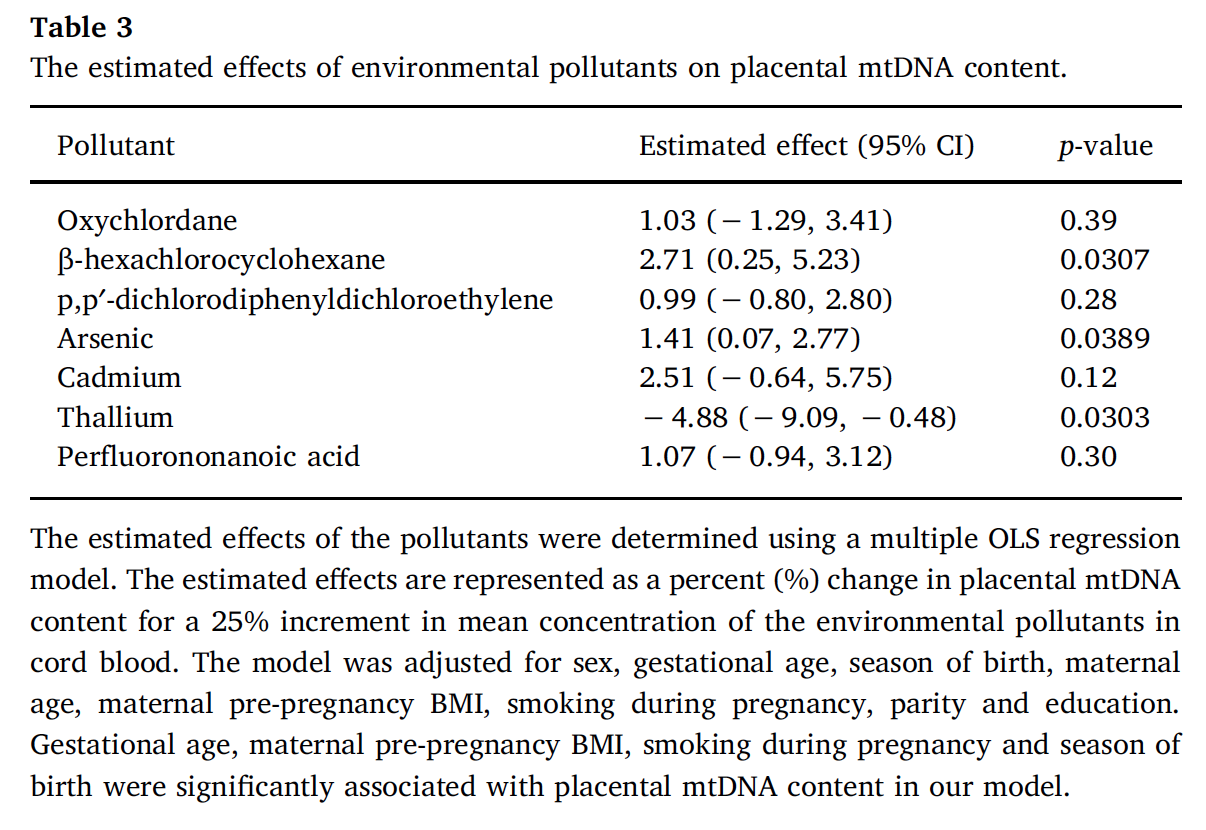
Figure 3.18: Final results from Vriens et al. 2017