2.1 Data pre-processing
Before getting into the actual analysis of the mixture it is important to carefully assess each component independently. Environmental exposures such as chemicals or pollutants, but also indicators of greenness, noise, or temperature, share important characteristics that should be carefullly addressed.
Skewedness and variance. Exposures are often non-negative and heavily skewed on the right due to the presence of outliers and to the fact that they are strictly non-negative. For this reason, it is usually recommended to log-transform these exposures. Nevertheless, when such operation is taken into account, researchers have to deal with decisions on how to treat eventual zero-values that do not necessarily represent missing data (see third bullet).
Centering and standardizing exposures. Mixture components tend to have different and difficult-to-compare scales and variability, even within the same family of exposures. Since these exposures will be eventually evaluated together, centering and standardizing the covariates will allow comparability and improve interpretation of statistical findings.
Zero values. It is relatively common, when evaluating large mixtures of environmental exposures, to encounter one or more covariates with a considerable amount of values equal to 0. How to deal with such zero-values will have important consequences on the implementation and interpretation of statistical approaches for mixtures. The first question to consider is what these zero values represent: specifically, are they “real zeros” (i.e. the individuals had no exposure to a given chemical), or do they represent non-detected values (i.e. the individual had a low level of exposure that we were not able to detect)? In the first case, the values will have to be treated as an actual zero, with important implications for the analysis. In the second case, non-detected values are usually imputed to a predefined value (several approaches are available) and the covariate can be treated as continuous. We will briefly deal with this when talking about zero-inflated covariates in Section 6.
Missing values. Finally, it is important to evaluate the percentage of missing values for each exposure in our mixture. Most techniques that allow evaluating the joint effect of several covariates, including regresison models, will generallyrequire a complete-case analysis. As such, an individual with just one missing values in one of the several mixture components, will be excluded from the whole analyses. If the proportion of missingness is not too high (10-15%), multiple imputation techniques can be used, even though the user should be aware that most advanced methodologies might not be fully integrated withing a multiple implementation procedure. If the percentage of missingness is too high, there is not too much to be done, and we will have to decide whether to give up the covariate (excluding it from the mixture), or reduce the sample size (excluding all individual with missing values on that component)
The dataset used in the illustrative example includes simulated covariates where this pre-processing steps have been already completed ( all values are greater than 0, no missing data are present, covariates are log-transofmred and standardized).
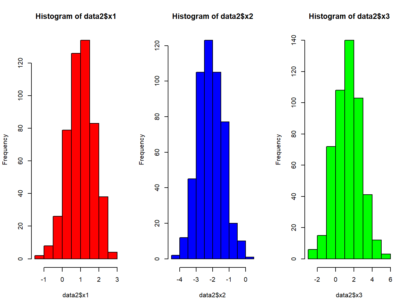
Figure 2.1: Histogram of three mixture components in the simulated data
To conduct a thorough exploratory analysis of environmental mixtures, especially when several covariates are of interest, we encourage the use of the R package rexposome, presented here