2.4 Cluster analysis

While a principal components analysis can be seen as a way to identify subgroups of exposures (the columns of the mixture matrix) within the mixture based on their correlation structure, another useful exploratory analysis consists in identifying subgroups of individuals (the rows of the data) that share similar exposure profiles. This is commonly done with cluster analysis. Like PCA, cluster analysis requires complete data and standardized variables. To group individuals, a distance measure must be identified, with several options available from standard euclidean distance to distances based on the correlations structure.

2.4.1 K-means clustering

The most common approach to partition the data into clusters is an unsupervised approach called k-means clustering. This method classifies objects in \(k\) groups (i.e., clusters), so that individuals within the same cluster are as similar as possible, while individuals from different clusters are as dissimilar as possible. To achieve that, clusters are defined in a way that minimizes within-cluster variation. A simple algorithm for k-clustering proceeds as follow

Pre-specify \(k\), the number of clusters
Select \(k\) random individuals as center for each cluster and define the centroids, vectors of length \(p\) that contain the means of all variables for the observation in the cluster. In our context, the \(p\) variables are the components of our mixture of interest
Define a distance measure. The standard choice is the euclidean distance defined as \((x_i-\mu_k)\) i, for each individual in the study (\(x_i\)) and each cluster center (\(\mu_k\))
Assign each individual to the closest centroid
For each of the \(k\) clusters update the cluster centroid by calculating the new mean values of all the data points in the cluster
Iteratively update the previous 2 steps until the the cluster assignments stop changing or the maximum number of iterations is reached. By default, the R software uses 10 as the default value for the maximum number of iterations

This simple algorithm minimizes the total within-cluster variation, defined for each cluster \(C_k\) as the sum of squared euclidean distances within that cluster \(W(C_k)=\sum_{x_i\in C_k}(x_i-\mu_k)^2\)

Since k-mean clustering requires the user to specify the number of groups, it is important to assess the optimal number of groups. A simple technique is to use the elbow method, similar to the one presented for PCA, which consists in plotting the within-cluster sum of squares versus the number of clusters, and locating the bend in the plot.

Several alternative approaches exist, including:

Hierarchical clustering
Model-based clustering
Density-based clustering
Fuzzy clustering

A simple introduction to each of these approaches can be found here. Model-based clustering, in particular, might represent an ideal alternatives in the presence of additional layers of complexity such as mixtures of both binary and continuous predictors, or missing data. The approach is implemented and well documented in the R package VarSelLCM

2.4.2 K-means in R

We can compute k-means in R with the kmeans function within the cluster package. Here we are selecting 3 groups, also using the nstart option that will attempts multiple initial configurations (here 20) and report the best one.

k3 <- kmeans(X, centers = 3, nstart = 20)

The option fviz_cluster provides a nice graphical representation of the groupings. If there are more than two variables fviz_cluster will perform principal component analysis (PCA) and plot the data points according to the first two principal components that explain the majority of the variance.

fviz_cluster(k3, data = X)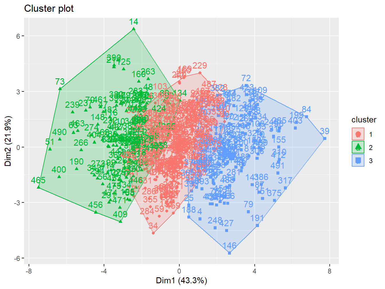

Figure 2.11: Cluster analysis with 3 groups in the simulated data

Here we can test more number of clusters

p1 <- fviz_cluster(k2, geom = "point", data = X) + ggtitle("k = 2")
p2 <- fviz_cluster(k3, geom = "point",  data = X) + ggtitle("k = 3")
p3 <- fviz_cluster(k4, geom = "point",  data = X) + ggtitle("k = 4")
p4 <- fviz_cluster(k5, geom = "point",  data = X) + ggtitle("k = 5")

grid.arrange(p1, p2, p3, p4, nrow = 2)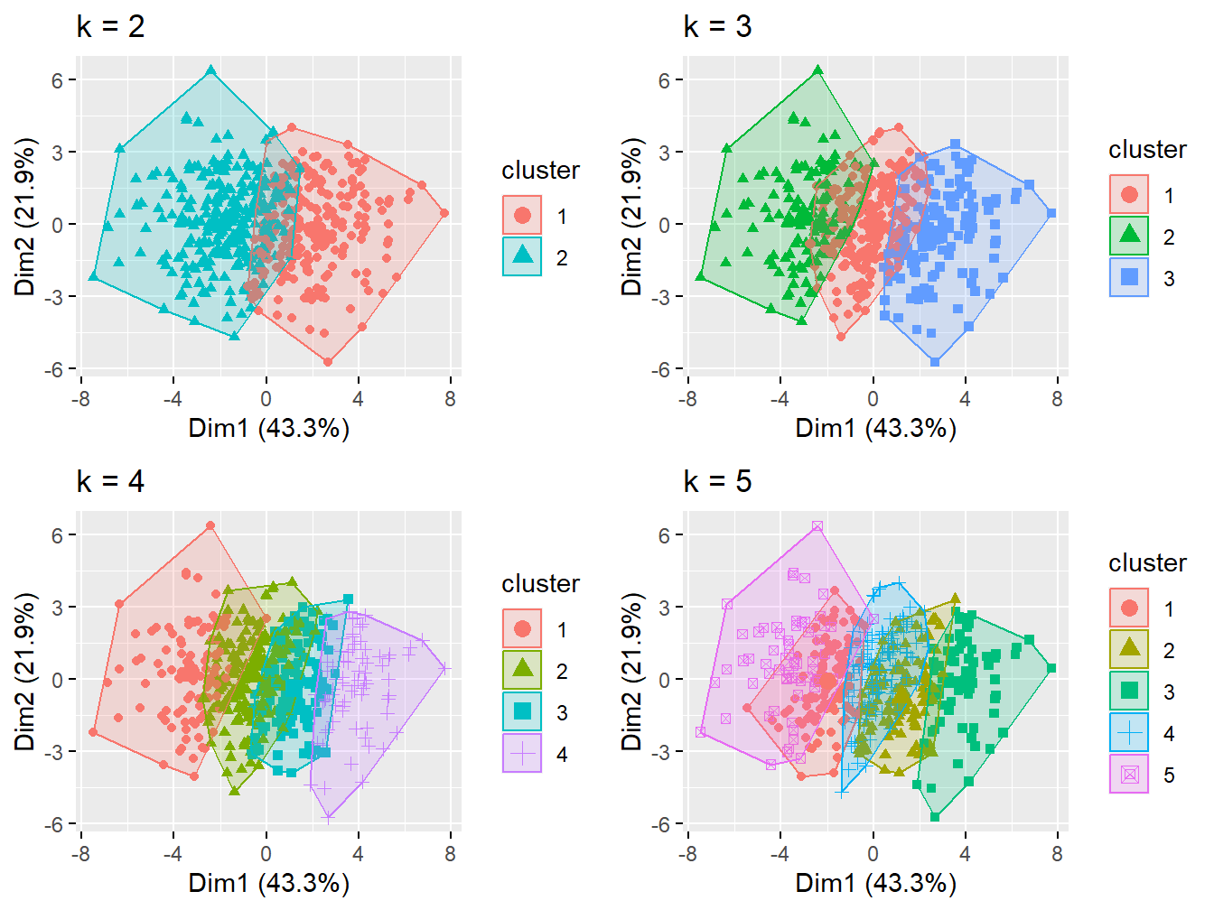

Figure 2.12: Cluster analysis with 2-5 groups

The elbow plot can tell us how many groups optimally classify individuals. This figure shows that 2 custers might be enough.

set.seed(123)
fviz_nbclust(X, kmeans, method = "wss")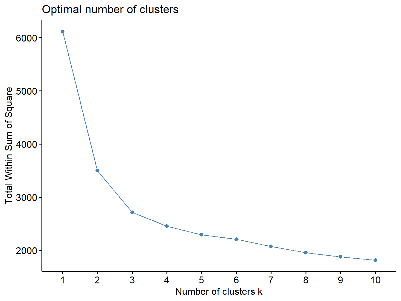

Figure 2.13: Elbow plot

2.4.3 Cluster analysis to simplify descriptive statistics presentation

One of the advantages of clustering individuals is to provide a better presentation of descriptive statistics and univariate associations with other covariates in the dataset prior to formal analysis (what is commonly done in table 1 of a scientific manuscript). First, let’s define the exposure profiles by evaluating the distribution of original exposures in the clusters (Table 2.3).

Table 2.3: Exposure distributions by clusters in the simulated data
	1	2	Overall
	(N=236)	(N=264)	(N=500)
x1
Mean (SD)	1.04 (0.718)	1.01 (0.684)	1.02 (0.699)
Median [Min, Max]	1.04 [-1.18, 2.49]	1.02 [-0.936, 2.89]	1.03 [-1.18, 2.89]
x2
Mean (SD)	-2.05 (0.765)	-2.18 (0.759)	-2.12 (0.764)
Median [Min, Max]	-2.10 [-4.32, 0.193]	-2.23 [-4.01, -0.291]	-2.14 [-4.32, 0.193]
x3
Mean (SD)	2.48 (0.885)	0.291 (0.907)	1.32 (1.41)
Median [Min, Max]	2.36 [0.993, 5.43]	0.511 [-2.33, 1.83]	1.33 [-2.33, 5.43]
x4
Mean (SD)	3.49 (0.867)	1.33 (0.889)	2.35 (1.39)
Median [Min, Max]	3.39 [1.93, 6.36]	1.51 [-1.36, 2.92]	2.32 [-1.36, 6.36]
x5
Mean (SD)	1.86 (1.03)	-0.645 (1.04)	0.537 (1.62)
Median [Min, Max]	1.81 [-0.311, 4.85]	-0.459 [-4.22, 1.42]	0.504 [-4.22, 4.85]
x6
Mean (SD)	1.52 (0.892)	0.326 (0.815)	0.891 (1.04)
Median [Min, Max]	1.50 [-0.564, 3.76]	0.356 [-2.12, 2.25]	0.833 [-2.12, 3.76]
x7
Mean (SD)	1.51 (0.556)	1.15 (0.490)	1.32 (0.552)
Median [Min, Max]	1.51 [0.216, 2.94]	1.18 [-0.356, 2.50]	1.33 [-0.356, 2.94]
x8
Mean (SD)	3.39 (0.737)	2.08 (0.767)	2.70 (0.999)
Median [Min, Max]	3.31 [1.65, 5.92]	2.10 [-0.268, 4.84]	2.69 [-0.268, 5.92]
x9
Mean (SD)	1.45 (0.529)	1.21 (0.571)	1.32 (0.564)
Median [Min, Max]	1.43 [0.0496, 2.70]	1.25 [-0.328, 2.98]	1.34 [-0.328, 2.98]
x10
Mean (SD)	3.46 (0.690)	2.86 (0.683)	3.14 (0.748)
Median [Min, Max]	3.42 [1.69, 5.26]	2.81 [1.07, 4.66]	3.13 [1.07, 5.26]
x11
Mean (SD)	5.61 (0.638)	4.81 (0.674)	5.19 (0.769)
Median [Min, Max]	5.53 [3.98, 7.80]	4.80 [2.62, 6.71]	5.21 [2.62, 7.80]
x12
Mean (SD)	0.466 (0.337)	0.493 (0.347)	0.481 (0.342)
Median [Min, Max]	0.443 [-0.429, 1.15]	0.507 [-0.481, 1.49]	0.483 [-0.481, 1.49]
x13
Mean (SD)	0.530 (0.348)	0.578 (0.348)	0.555 (0.349)
Median [Min, Max]	0.514 [-0.371, 1.42]	0.570 [-0.355, 1.65]	0.552 [-0.371, 1.65]
x14
Mean (SD)	1.79 (0.549)	0.881 (0.562)	1.31 (0.719)
Median [Min, Max]	1.79 [0.373, 3.55]	0.879 [-1.29, 2.64]	1.31 [-1.29, 3.55]
We see that individu	als in the first cluste	r have higher exposure l	evels to most of the included contaminants, so we could define cluster 1 as “high” and cluster 2 as “low” exposure. Next, we can use the clusters to assess the distribution of outcome and covariates by clustering (Table 2.4).

Table 2.4: Covariate distributions by clusters in the simulated data
	1	2	Overall
	(N=236)	(N=264)	(N=500)
Outcome
Mean (SD)	4.19 (0.619)	3.64 (0.569)	3.90 (0.653)
Median [Min, Max]	4.17 [2.66, 6.00]	3.62 [2.25, 5.22]	3.87 [2.25, 6.00]
Poverty index
Mean (SD)	2.26 (1.59)	1.90 (1.63)	2.07 (1.62)
Median [Min, Max]	2.18 [-1.87, 7.62]	1.87 [-2.47, 5.95]	2.08 [-2.47, 7.62]
Age
Mean (SD)	46.4 (18.8)	14.4 (17.9)	29.5 (24.3)
Median [Min, Max]	45.2 [1.01, 102]	15.1 [-38.3, 54.3]	28.6 [-38.3, 102]

We see that both z1, z2, z3, as well as the outcome are higher among individuals in cluster 1, who are characterized by the exposure profile presented in the previous table.

Other potential applications of cluster analysis in environmental epidemiology exist (see for example Austin et al. (2012)).

References

Austin, Elena, Brent Coull, Dylan Thomas, and Petros Koutrakis. 2012. “A Framework for Identifying Distinct Multipollutant Profiles in Air Pollution Data.” Environment International 45: 112–21.