5.1 Bayesian Kernel Machine Regression
5.1.1 Introduction
Bayesian Kernel Machine Regression (BKMR) is designed to address, in a flexible non-parametric way, several objectives such as detection and estimation of an effect of the overall mixture, identification of pollutant or group of pollutants responsible for observed mixture effects,visualizing the exposure-response function, or detection of interactions among individual pollutants. The main idea of BKMR is to model exposure through means of a kernel function. Specifically, the general modeling framework is
\[Y_i=h(z_{i1},…,z_{iM})+βx_i+\epsilon_i\]
where \(Y_i\) is a continuous, normally distributed health endpoint, \(h\) is a flexible function of the predictor variables \(z_{i1},…,z_{iM}\), and \(x_i\) is a vector of covariates assumed to have a linear relationship with the outcome
There are several choices for the kernel function used to represent \(h\). The focus here is on the Gaussian kernel, which flexibly captures a wide range of underlying functional forms for h and can accommodate nonlinear and non-additive effects of the multivariate exposure. Specifically, the Gaussian kernel implies the following representation for \(h\):
\[K_{vs}(z_i,z_j)=exp\{-\sum_{M}r_m(z_{im}-z_{jm})^2\}\]
Intuitively, the kernel function shrinks the estimated health effects of two individuals with similar exposure profiles toward each other. The weights \(r_m\) present the probability that each exposure is important in the function, with \(r_m=0\) indicating that there is no association between the \(m^{th}\) exposure and the outcome. By allowing some weights to be 0, the method is implicitly embedding a variable selection procedure. This can also integrate information on existing structures among exposures (e.g. correlation clusters, PCA results, similar mechanisms …) with the so-called hierarchical variable selection, which estimates the probability that each group of exposures is important, and the probability that, given a group is important, each exposure in that group is driving that group-outcome association.
5.1.2 Estimation
BKMR takes its full name from the Bayesian approach used for estimating the parameters. The advantages of this include the ability of estimating the importance of each variable (\(r_m\)) simultaneously, estimating uncertainties measures, and easily extending the estimation to longitudinal data. Since the estimation is built within an iterative procedure (MCMC), variable importance are provided in terms of Posterior Inclusion Probability (PIP), the proportion of iterations with \(r_m>0\). Typically, several thousands of iterations are required.
The bkmr R package developed by the authors makes implementation of this technique relatively straightforward. Using our illustrative example, the following chunk of code presents a set of lines that are required before estimating a BKMR model. Specifically, we are defining the object containing the mixture (\(X_{1}-X_{14}\)), the outcome (\(Y\)), and the confounders (\(Z_1-Z_3\)). We also need to generate a seed (we are using an iterative process with a random component) and a knots matrix that will help speeding up the process. This final step is very important as the model estimation can be extremely long (the recommendation is to use a number of knots of more or less n/10).
mixture<-as.matrix(data2[,3:16])
y<-data2$y
covariates<-as.matrix(data2[,17:19])

set.seed(10)
knots100  <- fields::cover.design(mixture, nd = 50)$design
The actual estimation of a BKMR model is very simple and requires one line of R code. With the following lines we fit a BKMR model with Gaussian predictive process using 100 knots. We are using 1000 MCMC iterations for the sake of time, but a final analysis should be run on a much larger number of samples, up to 50000. Here we are allowing for variable selection, but not providing any information on grouping.
temp <-  kmbayes(y=y, Z=mixture, X=covariates, iter=1000, verbose=FALSE,
varsel=TRUE, knots=knots100)| variable | PIP |
|---|---|
| x1 | 0.110 |
| x2 | 0.082 |
| x3 | 0.000 |
| x4 | 0.000 |
| x5 | 0.072 |
| x6 | 0.142 |
| x7 | 0.000 |
| x8 | 0.336 |
| x9 | 0.062 |
| x10 | 0.400 |
| x11 | 0.188 |
| x12 | 0.818 |
| x13 | 0.080 |
| x14 | 0.158 |
The ExtractPIPs() command will show one of the most important results, the posterior inclusion probabilities, shown in Table 5.1. We can interpret this output as the variable selection part, in which we get information on the importance of each covariate in defining the exposures-outcome association. In descending order, the most important contribution seems to come from \(X_{12}, X_{6}, X_{10}, X_{2}, X_{14}, X_{11}\). This is in agreement with Elastic Net and WQS, which also identified \(X_{12}\) and \(X_6\) as the most important contributors. Also note that within the other cluster we haven’t yet been able to understand who the bad actor is, if any exists.
5.1.3 Trace plots and burning phase
Since we are using several iterations it is important to evaluate the convergence of the parameters. These can be checked by looking at trace plots (what we expect here is some kind of random behaving around a straight line). What we generally observe is an initial phase of burning, which we should remove from the analysis. Here, we are removing the first 100 iterations and this number should be modify depending on the results of your first plots (Figures 5.1 and 5.2).
sel<-seq(0,1000,by=1)TracePlot(fit = temp, par = "beta", sel=sel)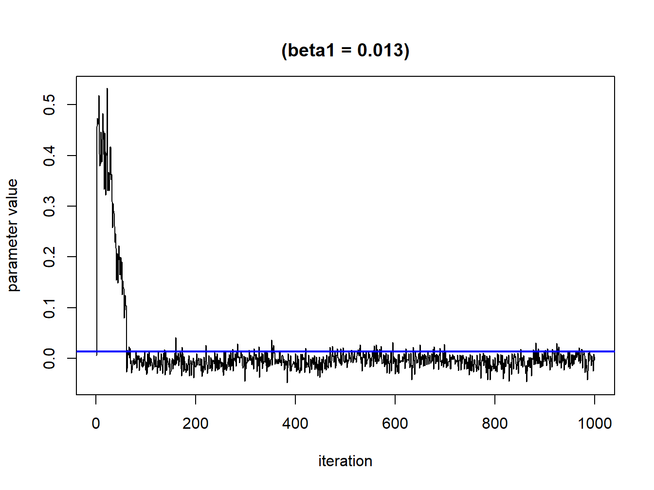
Figure 5.1: Convergence plot for a single parameter without exclusions
sel<-seq(100,1000,by=1)TracePlot(fit = temp, par = "beta", sel=sel)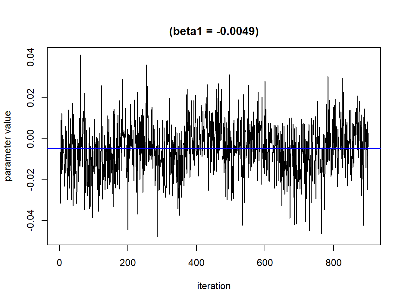
Figure 5.2: Convergence plot for a single parameter after burning phase exclusion
5.1.4 Visualizing results
After estimation of a BKMR model, which is relatively straightforward and just requires patience throughout iterations, most of the work will consist of presenting post-estimation figures that can present the complex relationship between the mixture and the outcome. The R package includes several functions to summarize the model output in different ways and to visually display the results.
To visualize the exposure-response functions we need to create different dataframes with the predictions that will be then graphically displayed with ggpolot.
pred.resp.univar <- PredictorResponseUnivar(fit=temp, sel=sel,
                                            method="approx")

pred.resp.bivar  <- PredictorResponseBivar(fit=temp,  min.plot.dist = 1,
                                           sel=sel,  method="approx")

pred.resp.bivar.levels <- PredictorResponseBivarLevels(pred.resp.df=
                        pred.resp.bivar,   Z = mixture, both_pairs=TRUE,
                        qs = c(0.25, 0.5, 0.75))

risks.overall <- OverallRiskSummaries(fit=temp, qs=seq(0.25, 0.75, by=0.05),
                                      q.fixed = 0.5, method = "approx",
                                      sel=sel)

risks.singvar <- SingVarRiskSummaries(fit=temp, qs.diff = c(0.25, 0.75),
                                      q.fixed = c(0.25, 0.50, 0.75),
                                      method = "approx")

risks.int <- SingVarIntSummaries(fit=temp, qs.diff = c(0.25, 0.75),
                                 qs.fixed = c(0.25, 0.75))
The first three objects will allow us to examine the predictor-response functions, while the next three objects will calculate a range of summary statistics that highlight specific features of the surface.
5.1.4.1 Univariate dose-responses
One cross section of interest is the univariate relationship between each covariate and the outcome, where all of the other exposures are fixed to a particular percentile (Figure 5.3). This can be done using the function PredictorResponseUnivar. The argument specifying the quantile at which to fix the other exposures is given by q.fixed (the default value is q.fixed = 0.5).
ggplot(pred.resp.univar, aes(z, est, ymin = est - 1.96*se,
                             ymax = est + 1.96*se)) +
geom_smooth(stat = "identity") + ylab("h(z)") + facet_wrap(~ variable) 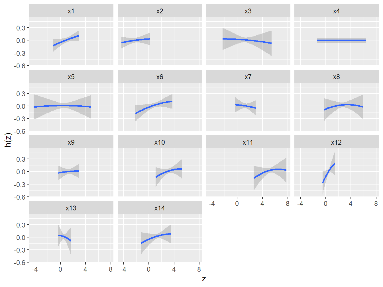
Figure 5.3: Univariate dose-response associations from BKMR in the simulated dataset
We can conclude from these figures that all selected covariates have weak to moderate associations, and that all dose-responses seem to be linear (maybe leaving some benefit of doubt to \(X_6\)).
5.1.4.2 Bivariable Exposure-Response Functions
This visualizes the bivariate exposure-response function for two predictors, where all of the other predictors are fixed at a particular percentile (Figure 5.4).
ggplot(pred.resp.bivar, aes(z1, z2, fill = est)) +
  geom_raster() +
  facet_grid(variable2 ~ variable1) +
  scale_fill_gradientn(colours=c("#0000FFFF","#FFFFFFFF","#FF0000FF")) +
  xlab("expos1") +
  ylab("expos2") +
  ggtitle("h(expos1, expos2)")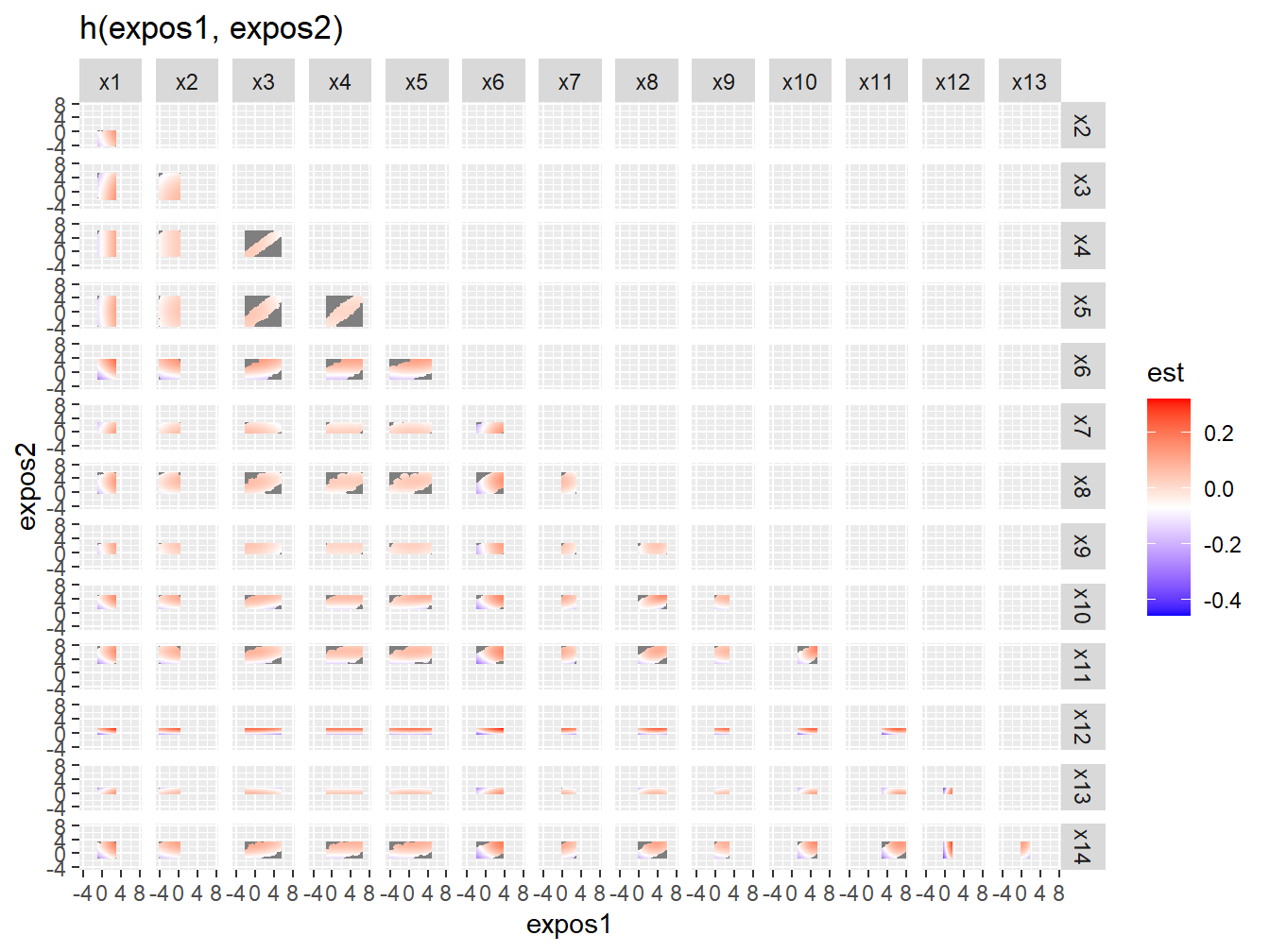
Figure 5.4: Bivariate exposure-response associations from BKMR in the simulated dataset
5.1.4.3 Interactions
Figure 5.4 might not be the most intuitive way of checking for interactions. An alternative approach is to investigate the predictor-response function of a single predictor in Z for the second predictor in Z fixed at various quantiles (and for the remaining predictors fixed to a specific value). These plots can be obtained using the PredictorResponseBivarLevels function, which takes as input the bivariate exposure-response function outputted from the previous command, where the argument qs specifies a sequence of quantiles at which to fix the second predictor. From the full set of combinations (Figure 5.5) we can easily select a specific one that we want to present, like the X6-X12 one (Figure 5.6).
ggplot(pred.resp.bivar.levels, aes(z1, est)) +
  geom_smooth(aes(col = quantile), stat = "identity") +
 facet_grid(variable2 ~ variable1) +
  ggtitle("h(expos1 | quantiles of expos2)") +
 xlab("expos1")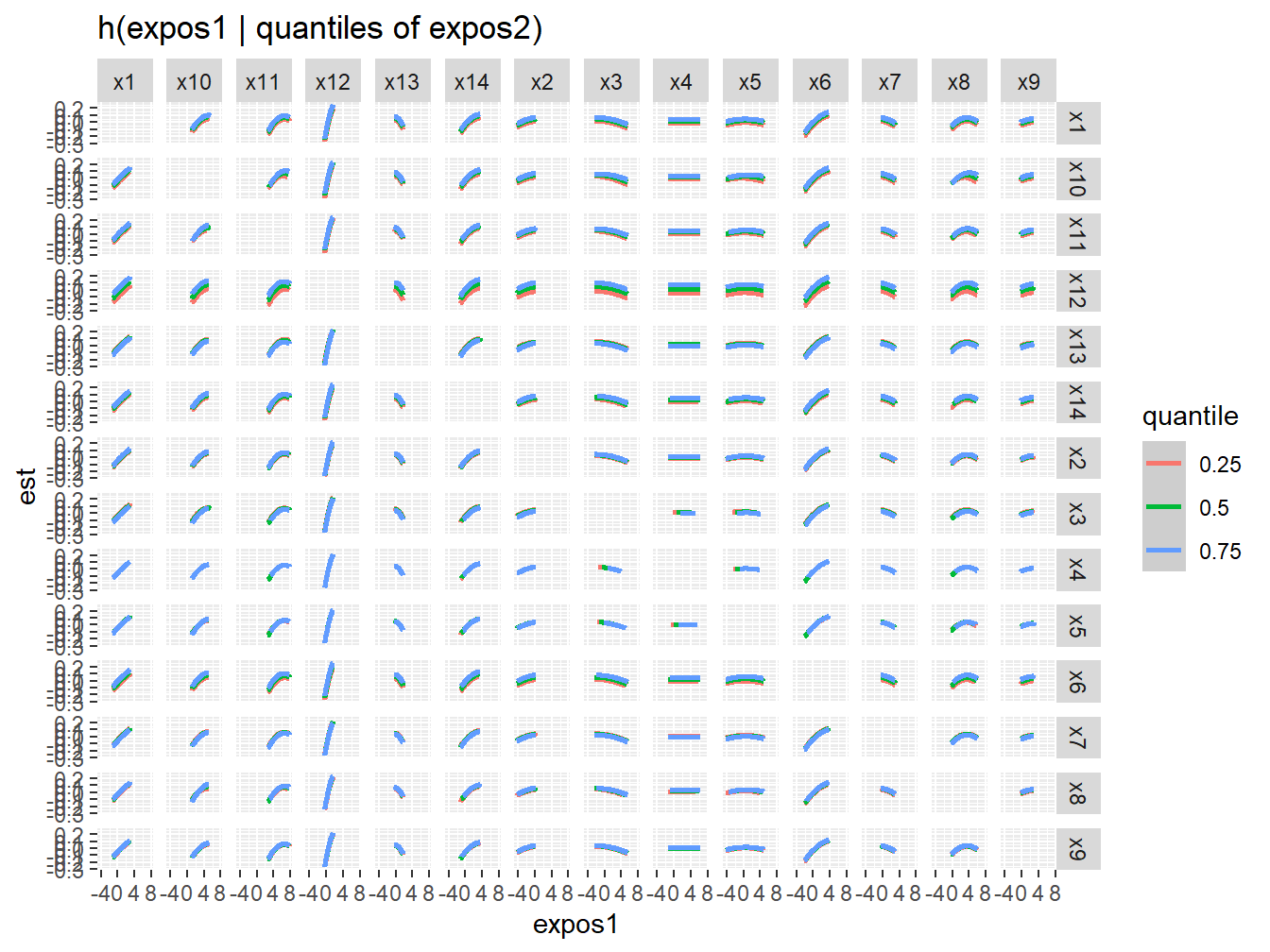
Figure 5.5: Qualitative interaction assessment from BKMR in the simulated dataset
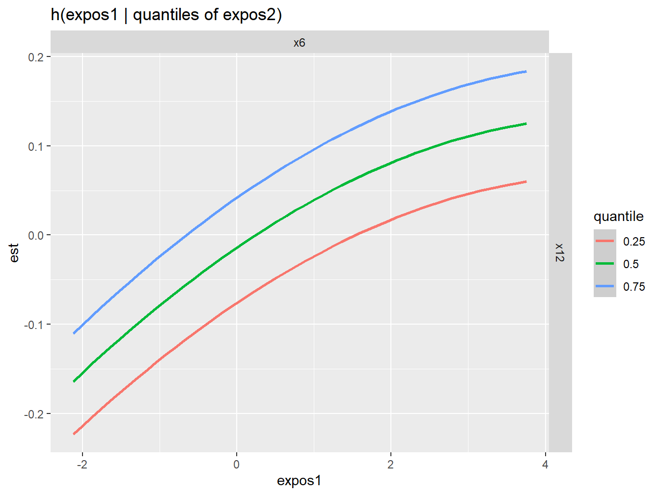
Figure 5.6: Qualitative interaction assessment between X6 and x12 from BKMR in the simulated dataset
These figures do not provide any evidence of interactions throughout the mixture. As we know, this is correct since no interactions were specified in the simulated dataset.
5.1.4.4 Overall Mixture Effect
Another interesting summary plot is the overall effect of the mixture, calculated by comparing the value of \(h\) when all of predictors are at a particular percentile as compared to when all of them are at their 50th percentile (Figure 5.7).
ggplot(risks.overall, aes(quantile, est, ymin = est - 1.96*sd,
                          ymax = est + 1.96*sd)) +
  geom_hline(yintercept=00, linetype="dashed", color="gray") +
geom_pointrange() + scale_y_continuous(name="estimate") 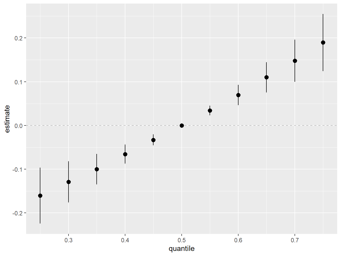
Figure 5.7: Overall Mixture Effect from BKMR in the simulated dataset
In agreement with WQS, higher exposure to the overall mixture is associated with higher mean outcome.
5.1.4.5 Single Variables effects
This additional function summarizes the contribution of an individual predictor to the response. For example, we may wish to compare the outcome when a single predictor in \(h\) is at the 75th percentile as compared to when that predictor is at its 25th percentile, where we fix all of the remaining predictors to a particular percentile (Figure 5.8).
ggplot(risks.singvar, aes(variable, est, ymin = est - 1.96*sd,
                          ymax = est + 1.96*sd, col = q.fixed)) +
       geom_hline(aes(yintercept=0), linetype="dashed", color="gray") +
       geom_pointrange(position = position_dodge(width = 0.75)) +
       coord_flip() + theme(legend.position="none")+scale_x_discrete(name="") +
scale_y_continuous(name="estimate") 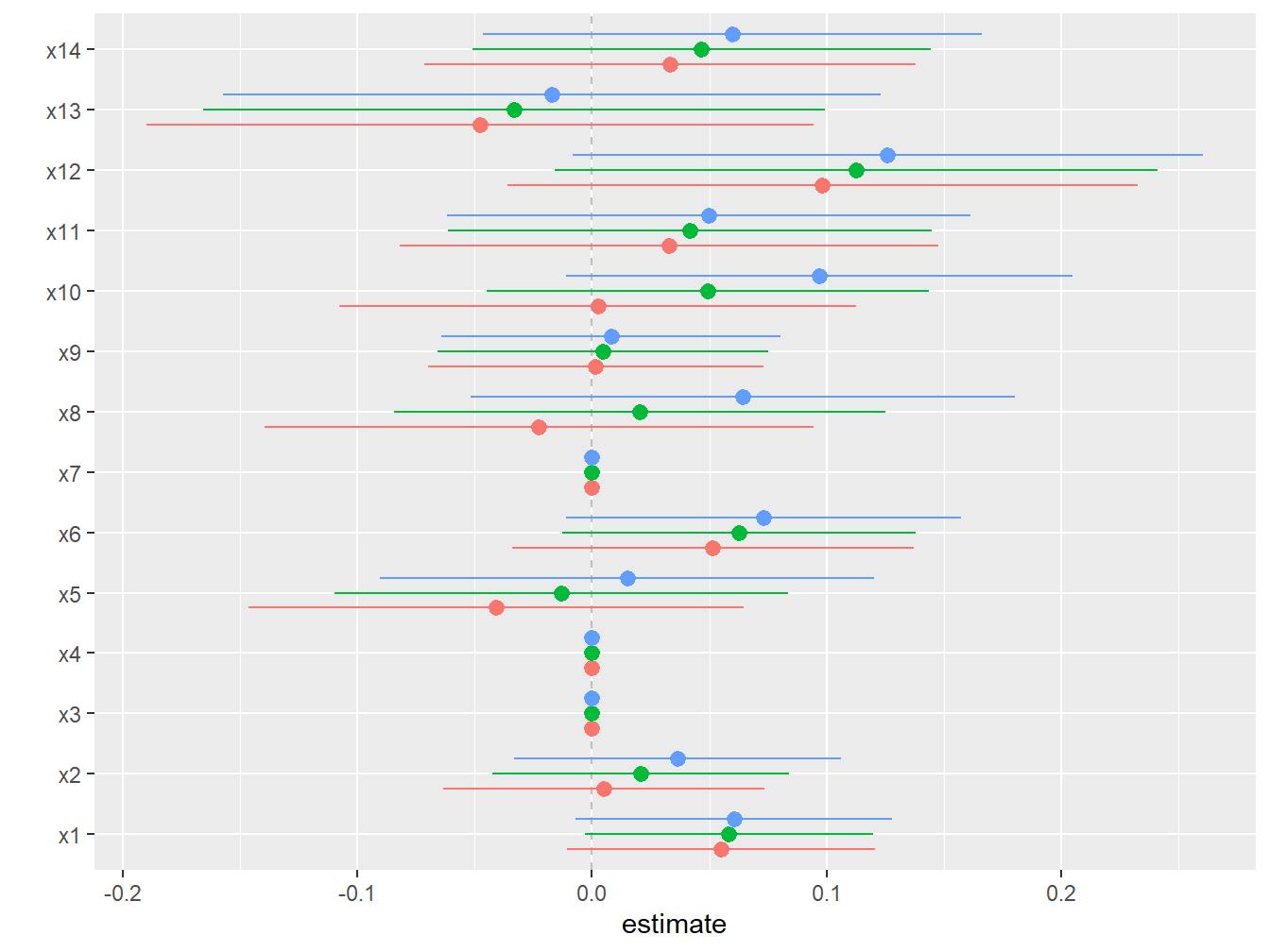
Figure 5.8: Individual effects from BKMR in the simulated dataset
5.1.4.6 Single Variable Interaction Terms
Finally, this function is similar to the latest one, but refers to the interaction of a single exposure with all other covariates. It attempts to represent an overall interaction between that exposure and all other components (Figure 5.9).
ggplot(risks.int, aes(variable, est, ymin = est - 1.96*sd,
                      ymax = est + 1.96*sd)) +
  geom_pointrange(position = position_dodge(width = 0.75)) +
  geom_hline(yintercept = 0, lty = 2, col = "brown") + coord_flip()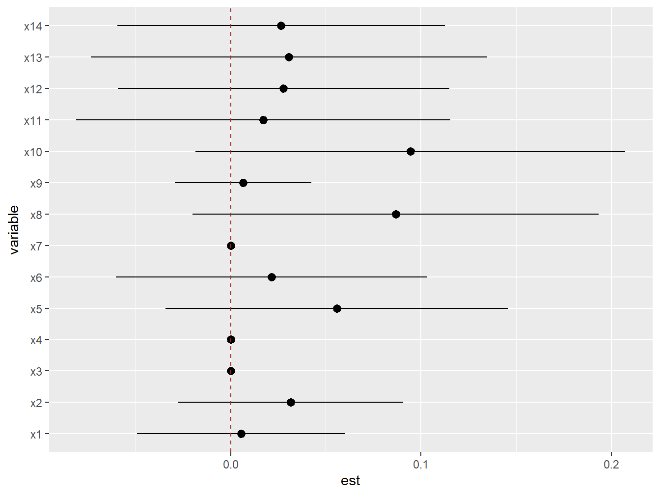
Figure 5.9: Individual interaction effects from BKMR in the simulated dataset
As we concluded before, this graph also leads us to conclude that we have no evidence of interaction for any covariate.
5.1.5 Hierarchical selection
The variable selection procedure embedded into BKMR can also operate within a hierarchical procedure. Using our example, we could for instance inform the model that there are highly correlated clusters of exposures. This will allow us to get an estimate of the relative importance of each cluster and of each exposure within it. The procedure is implemented as follows, where we are specifically informing the model that there is a cluster of three highly correlated covariates:
hier <-  kmbayes(y=y, Z=mixture, X=covariates, iter=1000,
                 verbose=FALSE, varsel=TRUE,  knots=knots100,
groups=c(1,1,2,2,2,1,1,1,1,1,1,1,1,1))| variable | group | groupPIP | condPIP |
|---|---|---|---|
| x1 | 1 | 1.000 | 0.0000000 |
| x2 | 1 | 1.000 | 0.0000000 |
| x3 | 2 | 0.044 | 0.3636364 |
| x4 | 2 | 0.044 | 0.4545455 |
| x5 | 2 | 0.044 | 0.1818182 |
| x6 | 1 | 1.000 | 0.0160000 |
| x7 | 1 | 1.000 | 0.0040000 |
| x8 | 1 | 1.000 | 0.0620000 |
| x9 | 1 | 1.000 | 0.0540000 |
| x10 | 1 | 1.000 | 0.0000000 |
| x11 | 1 | 1.000 | 0.0020000 |
| x12 | 1 | 1.000 | 0.4500000 |
| x13 | 1 | 1.000 | 0.1460000 |
| x14 | 1 | 1.000 | 0.2660000 |
Group PIPs, shown in Table 5.2, seem to point out that the cluster is somehow relevant in the dose-response association, and indicates that that \(X_4\) might be the most relevant of the three exposures.
5.1.6 BKMR Extensions
The first release of BKMR was only available for evaluating continuous outcomes, but recent work has extended its use to the context of binary outcomes, which are also integrated in the latest versions of the package. Domingo-Relloso et al. (2019) have also described how to apply BKMR with time-to-event outcomes. Additional extensions of the approach that could be of interest in several settings also include a longitudinal version of BKMR based on lagged regression, which can be used to evaluate time-varying mixtures (Liu et al. (2018)). While this method is not yet implemented in the package, it is important to note that similar results can be achieved by evaluating time-varying effects through hierarchical selection. In brief, multiple measurements of exposures can be included simultaneously in the kernel, grouping exposures by time. An example of this application can be found in Tyagi et al. (2021), evaluating exposures to phthalates during pregnancy, measured at different trimester, as they relate to final gestational weight. By providing a measure of group importance, group PIPs can here be interpreted as measures of relative importance of the time-windows of interest, thus allowing a better understanding of the timing of higher susceptibility to mixture exposures.
5.1.7 Practical considerations and discussion
To conclude our presentation of BKMR, let’s list some useful considerations that one should take into account when applying this methodology:
- As a Bayesian technique, prior information could be specified on the model parameters. Nevertheless this is not commonly done, and all code presented here is assuming the use of non-informative priors. In general, it is good to remember that PIP values can be sensitive to priors (although relative importance tends to be stable).
- Because of their sensitivity, PIP values can only be interpreted as a relative measure of importance (as ranking the importance of exposures). Several applied papers have been using thresholds (e.g. 0.5) to define a variable “important” but this interpretation is erroneous and misleading.
- The BKMR algorithm is more stable when it isn’t dealing with exposures on vastly different scales. We typically center and scale both the outcome and the exposures (and continuous confounders). Similarly, we should be wary of exposure outliers, and log-transforming exposures is also recommended.
- BKMR is operating a variable selection procedure. As such, a PIP of 0 will imply that the dose-response for that covariate is a straight line on zero. This does not mean that a given exposure has no effect on the outcome, but simply that it was not selected in the procedure. As a matter of fact, when an exposure has a weak effect on the outcome BKMR will tend to exclude it. As a consequence of this, the overall mixture effect will really present the overall effect of the selected exposures.
- As a Bayesian technique, BKMR is not based on the classical statistical framework on null-hypothesis testing. 95% CI are interpreted as credible intervals, and common discussions on statistical power should be avoided.
- Despite the estimation improvements through the use of knots as previously described, fitting a BKMR model remains time-demanding. In practice, you might be able to fit a BKMR model on a dataset of up to 10.000 individuals (still waiting few hours to get your results). For any larger dataset, alternative approaches should be considered.
- BKMR is a flexible non-parametric method that is designed to deal with complex settings with non-linearities and interactions. In standard situations, regression methods could provide a better estimation and an easier interpretation of results. In practical terms, you would never begin your analysis by fitting a BKMR model but only get to it for results validation or if alternative techniques were not sufficiently equipped to deal with your data.