Factor Analysis using method = minres
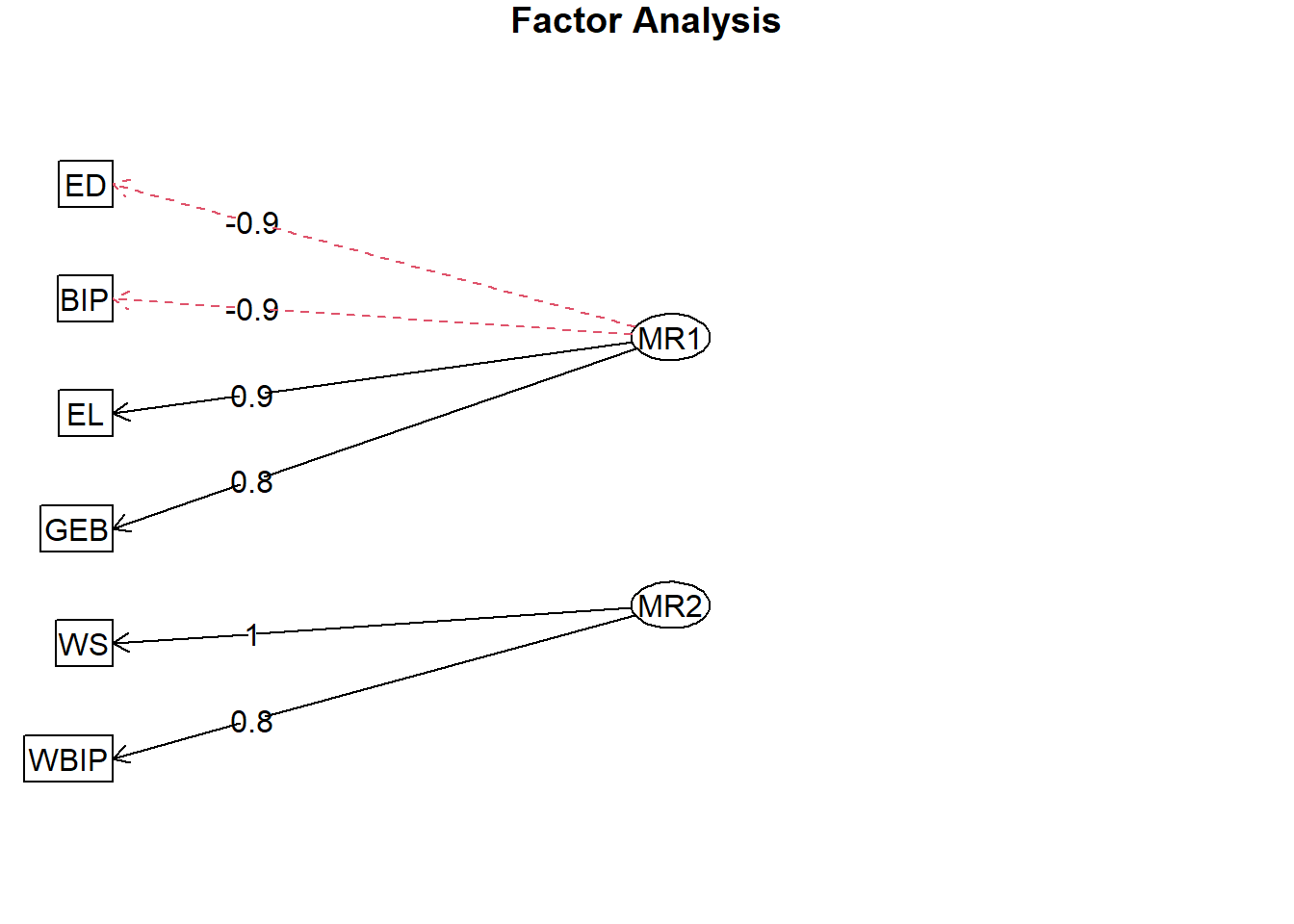
Call: fa(r = regionen_data, nfactors = 2, rotate = "varimax")
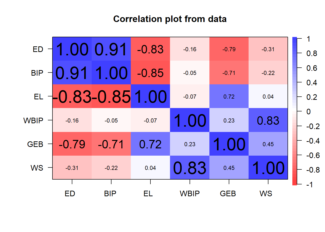
Standardized loadings (pattern matrix) based upon correlation matrix
item MR1 MR2 h2 u2 com
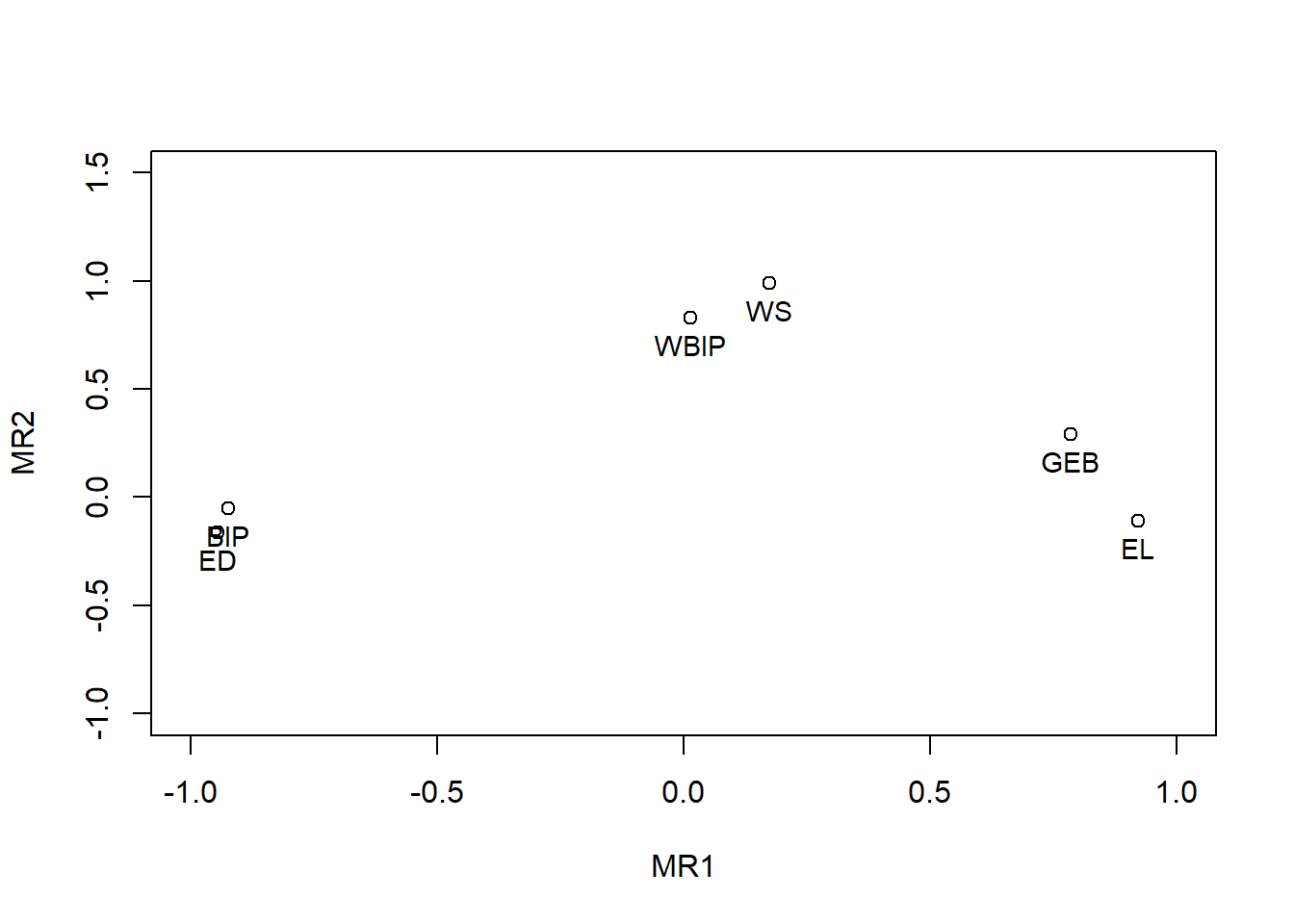
ED 1 -0.95 0.92 0.080 1.1
BIP 2 -0.92 0.86 0.142 1.0
EL 3 0.92 0.86 0.139 1.0
GEB 5 0.78 0.70 0.299 1.3
WS 6 0.99 1.01 -0.009 1.1
WBIP 4 0.83 0.69 0.309 1.0
MR1 MR2
SS loadings 3.25 1.79
Proportion Var 0.54 0.30
Cumulative Var 0.54 0.84
Proportion Explained 0.64 0.36
Cumulative Proportion 0.64 1.00
Mean item complexity = 1.1
Test of the hypothesis that 2 factors are sufficient.
df null model = 15 with the objective function = 5.99 with Chi Square = 48.88
df of the model are 4 and the objective function was 0.25
The root mean square of the residuals (RMSR) is 0.02
The df corrected root mean square of the residuals is 0.04
The harmonic n.obs is 12 with the empirical chi square 0.12 with prob < 1
The total n.obs was 12 with Likelihood Chi Square = 1.72 with prob < 0.79
Tucker Lewis Index of factoring reliability = 1.331
RMSEA index = 0 and the 90 % confidence intervals are 0 0.296
BIC = -8.22
Fit based upon off diagonal values = 1
Factor Analysis using method = minres
Call: fa(r = tlx_data, nfactors = 1, rotate = "varimax")
Standardized loadings (pattern matrix) based upon correlation matrix
V MR1 h2 u2 com
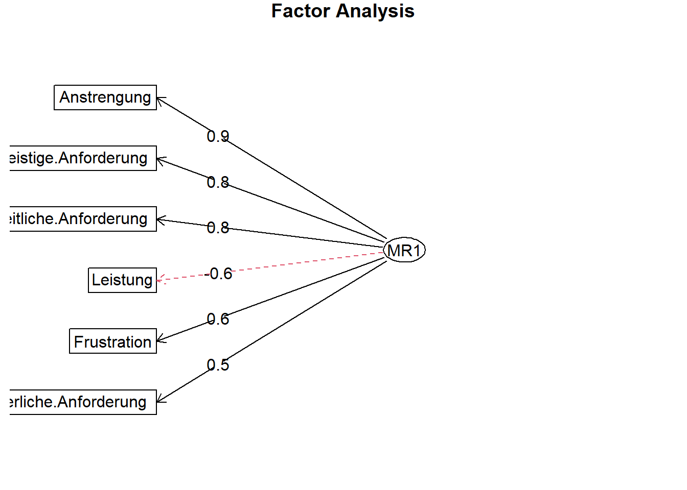
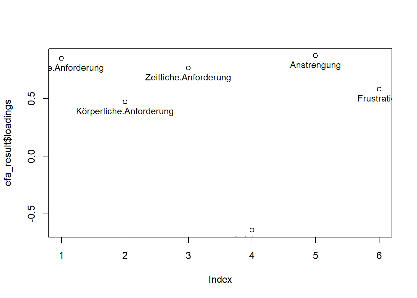
Anstrengung 5 0.87 0.76 0.24 1
Geistige.Anforderung 1 0.85 0.72 0.28 1
Zeitliche.Anforderung 3 0.76 0.58 0.42 1
Leistung 4 -0.64 0.41 0.59 1
Frustration 6 0.58 0.34 0.66 1
Körperliche.Anforderung 2 0.47 0.22 0.78 1
MR1
SS loadings 3.02
Proportion Var 0.50
Mean item complexity = 1
Test of the hypothesis that 1 factor is sufficient.
df null model = 15 with the objective function = 2.62 with Chi Square = 254.3
df of the model are 9 and the objective function was 0.1
The root mean square of the residuals (RMSR) is 0.04
The df corrected root mean square of the residuals is 0.05
The harmonic n.obs is 101 with the empirical chi square 4.46 with prob < 0.88
The total n.obs was 101 with Likelihood Chi Square = 9.37 with prob < 0.4
Tucker Lewis Index of factoring reliability = 0.997
RMSEA index = 0.017 and the 90 % confidence intervals are 0 0.115
BIC = -32.17
Fit based upon off diagonal values = 0.99
Measures of factor score adequacy
MR1
Correlation of (regression) scores with factors 0.94
Multiple R square of scores with factors 0.89
Minimum correlation of possible factor scores 0.78
# Diagramm der Faktorenladungen
fa.diagram(efa_result)
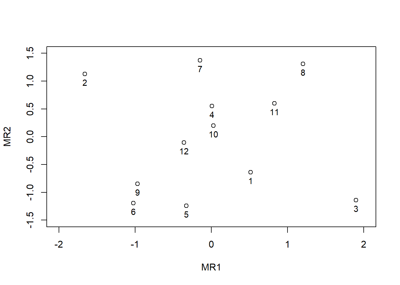
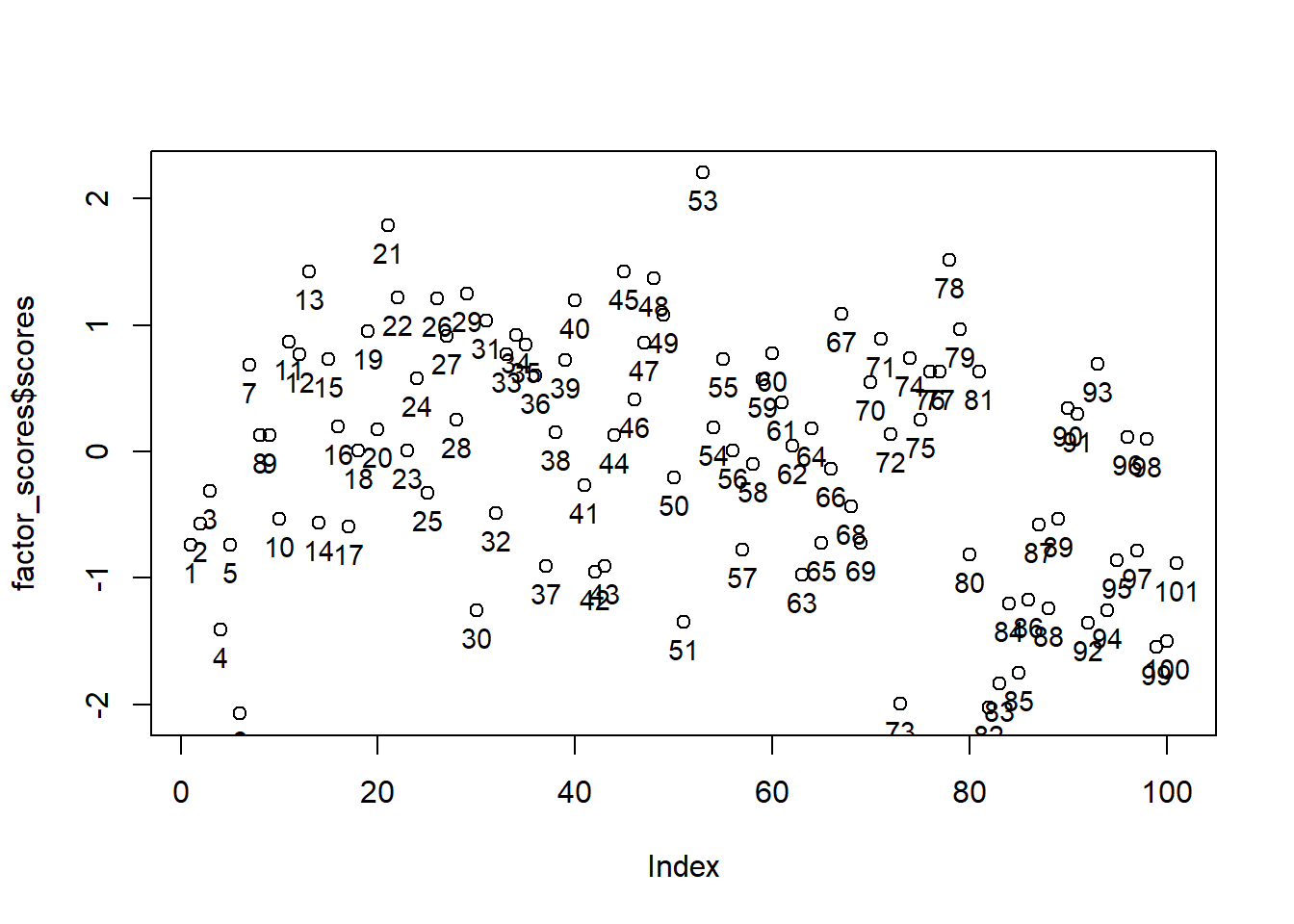
# Weitere Diagramme# Variablen im Faktorraumplot(factor_scores$scores)text(factor_scores$scores, labels =c(1:101), cex =0.9, pos =1, font =1, col ="black")
# Items im Faktorraum (Faktorwerte)plot(efa_result$loadings)text(efa_result$loadings, labels =colnames(tlx_data), cex =0.9, pos =1, font =1, col ="black")